The Effect of Hydrologic Model Calibration on Seasonal Streamflow Forecasts

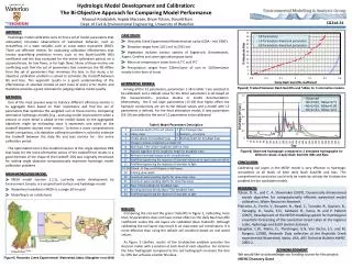
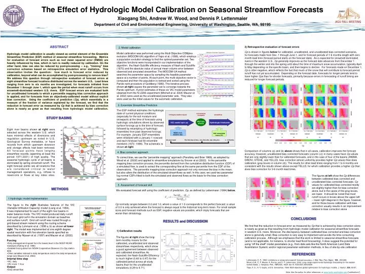
1. soil moisture snowpack 1/8 degree weather inputs streamflow North Fork Flathead (NOFOR) Stehekin (STEHE) Yellowstone (YELLO) Salmon (SALMO) INITIAL STATE VIC model spin up Hydrologic hindcasts NCDC met. station obs. ESP ensemble traces (30) Gunnison (BLMSA) Bruneau (BRUNE) Feather (OROVI) Animas (ANIMA) The first day of Dec., Jan.,Feb.,Mar.,Apr.,May,Jun. 10 years back 1 - 6 Months The Effect of Hydrologic Model Calibration on Seasonal Streamflow Forecasts Xiaogang Shi, Andrew W. Wood, and Dennis P. Lettenmaier Department of Civil and Environmental Engineering, University of Washington, Seattle, WA, 98195 ABSTRACT 2) Retrospective evaluation of forecast errors 2. Model calibration Cp is shown in figures below for calibrated, uncalibrated, and uncalibrated bias corrected scenarios, for forecasts made from Dec. 1 through June 1, and for forecast periods of 1-6 months length with zero month lead time (forecast period starts on the forecast date). As is expected for snowmelt dominated rivers in the western U.S., Cp generally improves as the forecast date advances from December 1 through the winter and into the spring until about the time of maximum snow accumulation, typically April to May depending on the specific basin, and then begins to decline. For forecasts made on December 1, Cp is often negative, which reflects the fact that much of the snow that will contribute to forecast period runoff has not yet accumulated. Depending on the forecast date, forecasts for longer periods tend to have higher Cps than for shorter forecasts, primarily because errors in forecasting of runoff timing are reduced for longer forecast periods. Model calibration was performed using the Multi Objective COMplex evolution (MOCOM-UA) algorithm of Yapo et al. (1998), which employs a population evolution strategy to find the optimal parameter set. Two objective functions were incorporated in our implementation of the algorithm: the Nash-Sutcliffe efficiency measure of Nash and Sutcliffe (1970) and the absolute value of annual mean volume error between observed and simulated streamflow. The MOCOM-UA method searches the parameter space by sampling the feasible parameter space at a number of points. At each point, the multi-objective vector is computed and then the population is ranked and sorted using the Pareto-rank procedure of Goldberg (1989). The iterative process shown at right causes the parameter set to converge towards the Pareto optimum. A priori estimates of these six VIC model parameters obtained from the N-LDAS experiment (Mitchell et al. 2004; Maurer et al. 2002) were used as the uncalibrated parameter sets. They also were used as the initial values for the automatic calibration. Hydrologic model calibration is usually viewed as central element of the Ensemble Streamflow Prediction (ESP) method of seasonal streamflow forecasting. Metrics for evaluation of forecast errors such as root mean squared error (RMSE) are heavily influenced by bias, which in turn is readily reduced by calibration. On the other hand, bias can also be reduced by post-processing -- e.g., “training” bias correction schemes based on retrospective simulation error statistics. This observation invites the question: how much is forecast error reduced by calibration, beyond what can be accomplished by post-processing to remove bias? We address this question through retrospective evaluation of forecast errors at eight streamflow forecast locations distributed across the western U.S.. Lead times ranging from zero to six months are investigated, for forecasts initiated from December 1 through June 1, which span the period when most runoff occurs from snowmelt-dominated western U.S. rivers. ESP forecast errors are evaluated both for uncalibrated forecasts to which a percentile mapping bias correction approach is applied, and for forecasts from an objectively-calibrated model without explicit bias correction. Using the coefficient of prediction (Cp), which essentially is a measure of the fraction of variance explained by the forecast, we find that the reduction in forecast error as measured by Cp that is achieved by bias correction alone is nearly as great as that resulting from hydrologic model calibration. 3. Ensemble Streamflow Prediction The ESP method estimates the hydrologic state of current physical conditions (especially for the soil moisture and snowpack) at the time of forecasts using hydrologic simulations driven by observed surface forcings up to the time of forecast, followed by resampling of hydrologic ensembles from past observed forcings. For example, January ESP ensembles were initialized with a January 1 nowcast and each hindcast had 30 ensemble members (1970 -1999). The schematic is shown at right. STUDY BASINS Eight river basins shown at right were selected across the western U.S. which have minimal effects of diversions and regulation upstream as noted in U.S. Geological Survey metadata, or have records from which upstream diversion and storage effects had been removed. All forecast points have lengthy streamflow records (spanning at least the period 1971-2001) of high quality. The seasonal hydrologic cycle of all basins is dominated by spring snowmelt runoff. The eight forecast points are all locations that are considered critical to water management operations, e.g., inflows to reservoirs or flows at key index sites. Comparison of columns (a) and (b) above shows that in all cases, calibration improves the forecast accuracy. However, uncalibrated bias corrected forecasts (column (c)) in many cases have Cp values that are only slightly lower than for calibrated forecasts, and in the case of four of the basins (ANIMA, OROVI, STEHE, and YELLO), bias correction almost uniformly provides higher Cp values than does calibration (gray boxes in column (d)). The results for other lead times ranging from 1 to 6 months are consistent with the results shown above except YELLO, for which calibration provides a higher Cp than does bias correction for 3-6 month lead times. 4. Bias correction approach To correct bias, we use the “percentile mapping” approach (Panofsky and Brier 1968), as adopted by Wood et al. (2002) and applied to streamflow simulations by Snover et al (2003). In the percentile mapping bias correction process, the percentile derived from the cumulative distribution function (CDF) of a simulated flow, is used to extract the corresponding flow at the same percentile from the CDF of the observations. The percentile mapping bias correction approach not only removes the bias in the mean, but also alters the distribution of the simulated streamflows as well. In this case, we used two-parameter log normal CDFs fitted to both the simulated and observed flows as the basis for the bias correction approach. The figures at left show the Cp differences between calibrated bias corrected and uncalibrated bias corrected forecasts. Cp values for calibrated bias corrected mostly are slightly higher than for bias correction alone, but in the cases of the gray boxes, are lower. It should be noted that most runoff occurs in boxes above the upper left – lower right diagonal in the figure, however, and for those boxes calibration with bias correction usually results in an improvement relative to bias correction alone • Assessment of forecast skill METHODS We evaluated forecast skill using the coefficient of prediction, Cp, as defined by Lettenmaier (1984) below. • Hydrologic model implementation Cp normally ranges between 0.0 and 1.0, where a value of 1.0 corresponds to the perfect forecast; a value of 0.0 is only achieved when the forecast is always equal to the historical long-term mean. For small sample sizes and forecast methods such as ESP, negative values are possible, which imply forecasts that are worse than climatology. The figure to the right illustrates features of the VIC (Variable Infiltration Capacity) model (Liang et al. 1994). It was implemented for each of the eight river basins in water balance mode. The VIC model produced daily runoff from each grid cell in the simulation domain as baseflow and surface runoff. Grid cell runoff was routed through a grid-based stream network using the routing scheme described by Lohmann et al. (1998 a, b) as shown at lower right. The model was implemented at one-eighth degree spatial resolution with five elevation bands specified as described by Nijssen et al. (1997) and Maurer et al. (2002). CONCLUSIONS RESULTS and DISCUSSION We find that the reduction in forecast error as measured by Cp that is achieved by bias correction alone is nearly as great as that resulting from hydrologic model calibration for seasonal streamflow forecasts in western U.S. rivers. Moreover, the discrepancy between calibrated bias corrected and bias correction alone is generally small. Bias correction is very easy to implement and avoids the time consuming calibration process. Although we emphasize that this work is limited to seasonal streamflow forecasts (and is not applicable, for instance, to shorter lead flood forecasting), it does suggest the potential for using “off the shelf” model parameters (e.g., from data sets like the North American Land Data Assimilation System) and/or regional parameter estimation methods, in lieu of site-by-site calibration • Calibration results The figures at right show the long-term monthly means for the calibrated, uncalibrated and observed streamflows respectively, which show a good agreement between observed and calibrated streamflow. As expected, the Nash-Sutcliffe Efficiency is much higher (0.83 to 0.97) for the calibrated period across all study basins than for the uncalibrated simulations (0.29 to 0.71). • Forcing • Daily averaged wind speed from the lowest level in the NCEP-NCAR reanalysis (Kalnay et al. 1996) • Gridded forcing data from NOAA Cooperative Observer (Co-Op) station data • Other variables indexed to daily temperature and/or the daily temperature range (see Maurer et al. 2002) • Internal time step • VIC: daily • VIC snow: 1 hour • Output • Daily streamflow REFERENCES Lettenmaier, D. P., 1984: Limitations on seasonal snowmelt forecast accuracy. J. Wat. Res. Plan. Mgmt., 108 , 255-269. Wood, A.W., E. P. Maurer, A. Kumar, and D. P. Lettenmaier, 2002: Long-range experimental hydrologic forecasting for the eastern United States. J. Geophys. Res., 107(D20), 4429, doi:10.1029/2001JD000659. Yapo, P. O., H. V. Gupta, and S. Sorooshian, 1998: Multi-objective global optimization for hydrologic models. J. Hydrol., 203, 83-97. Note: See the author for other references, or www.hydro.washington.edu (“publications”).