Download
1 / 1
10 likes | 134 Views
What is a Multi-Scale Analysis? Implications for Modeling Presence/Absence of Bird Species Kathryn M. Georgitis 1 , Alix I. Gitelman 1 , Don L. Stevens 1 , Nick Danz 2 , and JoAnn Hanowski 2 1 Department of Statistics Oregon State University Corvallis, Oregon

E N D
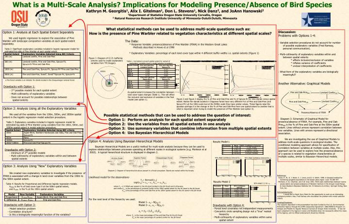
What is a Multi-Scale Analysis? Implications for Modeling Presence/Absence of Bird Species Kathryn M. Georgitis1, Alix I. Gitelman1, Don L. Stevens1, Nick Danz2, and JoAnn Hanowski2 1Department of Statistics Oregon State University Corvallis, Oregon 2 Natural Resources Research Institute University of Minnesota-DuluthDuluth, Minnesota Designs and Models for Aquatic Resource Surveys R82-9096-01 DAMARS Figure 1: Diagram of G.I.S. buffering scheme used to create explanatory variables from TM Imagery. Option 4: Analysis Using Bayesian Hierarchical Models Bayesian Hierarchical Models are a useful method for multi-scale analysis because they can be used to explore relationships between processes operating at different scales in ecological systems (e.g. Monleon et al 2002). A typical hierarchical structure is displayed in diagram 2. Diagram 2: Diagram of hierarchical structure present in a forest ecosystem. Stands are nested within the forests. Likelihood model for the observations- Yi.j~ Bernoulli(pi,j) Logit(pi,j) = a0,j + a1,j X1,i,j + a2,j X2,i,j where Yi,j =1 if PIWA was present in the ith stand located in the jth forest and 0 otherwise, and where X1,i,j is the percentage of Lowland Conifer at the 100m spatial extent for the ith stand in the jth forest X2,i,j is the percentage of Pine and Oak-Pine at the 100m spatial extent for the ith stand in the jth forest For the next level of the hierarchy we used: Model 1- a0 ~ N(mj,t) Model 2- a1, a2 ~ N(mj,t) mj = b0 + b1Z1,j +b2Z2,j where Z1,j is the mean percentage of Pine and Oak-Pine for the jth forest Z2,j is the mean percentage of Lowland conifer for the jth forest Chippewa Forest St.Croix Forest Superior Forest Chequamegon Forest Stand 3 Stand 3 Stand 1 Stand 2 Stand 3 Stand 2 Stand 2 Stand 1 Stand 4 Stand 6 Stand 5 Stand 4 Stand 3 Stand 2 Stand 4 Stand 1 Stand 1 Stand 5 What statistical methods can be used to address multi-scale questions such as: How is the presence of Pine Warbler related to vegetation characteristics at different spatial scales? The Data: * Response Variable: presence/absence of Pine Warbler (PIWA) in the Western Great Lakes -Methods described in Howe et al 1998 * Explanatory Variables: percentage of each land cover type within 4 different buffer widths i.e. spatial extents (Figure 1) Discussion: Problems with Options 1-4: - Variable selection procedures do not account for number of possible explanatory variables (Fred Ramsey, personal communication). - Multi-collinearity of explanatory variables within and between spatial extents * affects inclusion/exclusion of variables * inflates variance of coefficients * unclear interpretation of coefficients - What form of the explanatory variables are biologically meaningful? Another Alternative:Graphical Models Diagram 3: Schematic of Graphical Model for presence/absence of PIWA. For example, Pine and Oak-Pine500 is the % of Pine and Oak-Pine at the 500m spatial extent. Lines without arrows represent correlation between two variables. Lines with arrows represent a directional association. We are investigating the use of Graphical Models to address multi-scale questions in ecological studies. The conditional modeling approach allows for specification of correlation between variables at multiple scales. Also, this approach can be used to explore how the presence/absence of a species is related to vegetation characteristics at multiple scales, similar to Bayesian Hierarchical models. Option 1: Analysis at Each Spatial Extent Separately We used logistic regression to explore the association of Pine Warbler with landscape composition variables at each spatial extent separately. a:The forest variable is an indicator for stands located in the Chequamegon national forest. Drawbacks with Option 1: - 210 possible models for each spatial extent - Multi-collinearity of explanatory variables - Does not account for possible relationships between spatial extents 1000m 500m 100m Asspatial extent increases the correlation between land cover types changes (Table 1). This will affect the inclusion and exclusion of variables in the final model (see option 1). Pine and Oak-Pine500 Lowland Conifer500 Figure 2 and Figure 3 display the % of Pine and Oak-Pine and % of Spruce-fir for nine stands versus spatial extent. Notice the stands located in Chippewa forest have very different %’s of Pine and Oak-Pine (and Spruce-Fir) at the 100m scale but at the 5000m scale they have similar values. These figures raise the question perhaps it is the change in the % of Pine and Oak-Pine from one spatial extent to another that is what is important when trying to model the presence of Pine Warbler (see option 3). Lowland Conifer100 Pine and Oak-Pine100 • Option 2: Analysis Using all the Explanatory Variables • We used all the variables from the 100m, 500m, and 1000m spatial extent in the logistic regression model selection procedure. • Drawbacks with Option 2: • - minimum of 230 possible models • - Multi-collinearity of explanatory variables within and between • spatial extents Possible statistical methods that can be used to address the question of interest: Option 1: Perform an analysis for each spatial extent separately Option 2: Use the variables from all spatial extents in one analysis Option 3: Use summary variables that combine information from multiple spatial extents Option 4: Use Bayesian Hierarchical Models Presence/Absence of PIWA Results Model 1 95% Wald Confidence Interval for a1 95% Wald Confidence Interval for a2 Option 3: Analysis Using “New” Explanatory Variables We created new explanatory variables to investigate if the presence of PIWA is associated with a change in land cover variables from the 100m to the 500m spatial extent. Drawbacks with Option 3: - Model selection problem - Correlation structure? - Is this a biologically meaningful function of the variables? References: Howe, R. W., G. J. Niemi, S. J. Lewis, and D. A. Welsh. 1998. A standard method for monitoring songbird populations in the Great Lakes region. Loon 70:188-197. Monleon, V. A.I. Gitelman, and A.N. Gray. 2002. Multi-scale relationships between coarse woody debris and presence/absence of Western Hemlock in the Oregon Coast Range. In Case Studies in Bayesian Statistics Vol. VI Gatsonis et al (Eds.). Springer-Verlag, New York, Inc. Acknowledgements: I would like to thank Jerry Niemi for the opportunity to work on an interesting ecological problem. Also, Fred Ramsey who elucidated the problem with model selection criteria. Funding/Disclaimer: The research described in this presentation has been funded by the U.S. Environmental Protection Agency through the STAR Cooperative Agreement CR82-9096-01 Program on Designs and Models for Aquatic Resource Surveys at Oregon State University. It has not been subjected to the Agency's review and therefore does not necessarily reflect the views of the Agency, and no official endorsement should be inferred. Results Model 2 95% Wald C.I. for a0 • Drawbacks with Option 4: • - Forest level covariates not independent measurements • Concentric circle sampling design not a “true” nested hierarchy • Multi-collinearity of explanatory variables within same spatial extent