Download

1 / 63
630 likes | 750 Views
12 Mathematics B Topics - Semester 1 Exponential and Logarithmic Functions and Applications II Introduction to Integration I Periodic Functions and Applications III Optimisation Using Derivatives I Topics - Semester 2 Applied Statistical Analysis II Optimisation Using Derivatives II

E N D
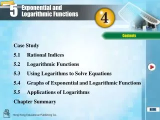
12 Mathematics B • Topics - Semester 1 • Exponential and Logarithmic Functions and Applications II • Introduction to Integration I • Periodic Functions and Applications III • Optimisation Using Derivatives I • Topics - Semester 2 • Applied Statistical Analysis II • Optimisation Using Derivatives II • Introduction to Functions III • Exponential and Logarithmic Functions and Applications III • Introduction to Integration III
Topic 9 Exponential and Logarithmic Functions and Applications II
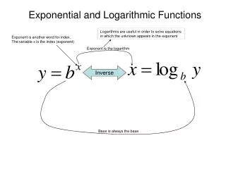
Definition of the exponential function ex • Graphs of and the relation between y=ax, y=logax for a=e and other values of a • Graphs of y=ekx for k≠0 • Applications of exponential and logarithmic functions • Development of algebraic models from appropriate data sets using logarithms and/or exponents • Derivatives of exponential and logarithmic functions for base e • Applications of the derivative of exponential functions • Use of logarithms to solve equations involving indices
SLE’s 2. Investigate life-related situations that can be modelled by simple exponential functions – e.g. applications of Newton’s Law of Cooling, concentration against time in chemistry, carbon dating in archaeology and decrease of atmospheric pressure with altitude. 3. Use a GC or computer software to investigate the shapes of exponential and logarithmic functions and their derivatives. 5. Investigate the role of indices (powers) in the establishment of formulae in financial matters such as compound interest, time required to repay a loan for given repayments and rate of interest. 6. Graph the derivative of a growth function or a decay function and interpret the result. 7. Investigate change such as radioactive decay, growth of bacteria, or growth of an epidemic, where the rate of change is proportional to the amount of material left or the current population size. 10.Consider the difference between assuming that running time is proportional to distance and assuming that log (running time) is proportional to log (distance); interpret the value of the constant of proportionality in the second model; world record times for either male or female athletes may be of interest in this context. 11.Investigate logarithmic scales, e.g. decibels, Moh’s scale of hardness, Richter scale and pH 12.Plot the logarithms of some apparent growth functions, e.g. car registrations over time, to produce a near linear graph 14.Plot the logarithm of the population of the Australia at censuses (a) from 1891 to 1933 (b0 from 1947 to 1971 and (c) from 1971 to 1991; recognize that the linear tendencies of the plot indicate power/exponential relationships in the original. 17.By graphing the logarithm of the distance of planets from the sun against the logarithm of the time of revolution about the sun, investigate the relationship between the variables.
Global Warming Global temperatures are rising. Observations collected over the last century suggest that the average land surface temperature has risen 0.45 – 0.6o C in the last century. The surface of the ocean has also been warming at a similar rate. About ⅔ of this warming took place between the turn of the century and 1940. Global temperatures declined slightly from the 1940’s through the 1970’s; but have risen more rapidly during the last 25 years than in the period before 1940.
Calling all Noahs! The burning of fossil fuels adds carbon dioxide to the atmosphere around the earth. This may be partly removed by biological reactions but the concentration of carbon dioxide is gradually increasing. This increase leads to a rise in the average temperature of the earth.
Although scientists have incontrovertible evidence that the surfaces of the land and oceans have been warming, some scientists are not yet convinced that the atmosphere is also warming. The satellite data do not show a warming trend, however the 1979 – 97 data series may be too short to show a trend in the atmospheric temperature. The absence of a warming trend in the satellite data provides an important caution that there is still much to learn about the global climate.
If the average temperature of the earth rises by about another 6oC from the present value, this would have a dramatic effect on the polar ice caps, winter temperatures etc. If the ice caps melt, there will be massive floods and a lot of the land mass would be submerged. The UK would disappear except for the tops of the mountains. Find a model of the above data and use it to predict when the earth’s temperature will be 7oC above its 1860 value. Should you start building an ark yet? Describe any limitations to your model.
The table shows the temperature rise over the last 100 years:
The types of graphs that we have looked at up until now have been of the form y = xn y = x3 y = x2
We are now going to look at graphs of the form y = ax Manually (no GC) draw the graph of y = 2x and y = (½)x Hint : Draw up a table of values of x from -4 to 4
We are now going to look at graphs of the form y = ax Manually (no GC) draw the graph of y = 2x and y = (½)x Hint : Draw up a table of values of x from -4 to 4
Applying Exponential and Logarithmic Functions A number of problems involving growth phenomena can be described using exponential and logarithmic functions. Such problems include economic growth (compound interest), biological growth, radioactive decay (negative growth), learning curves and sound intensities.
e.g. Compound interest is paid yearly at the rate of 20% p.a. on $10. The value of the investment after t years is given by the formula V = P(1+r)t where r = interest rate as a decimal and P = the original investment. Graph the value of the investment for the first 6 years. V=10 x 1.2 t
e.g. Jackie has just resumed athletics training after a season off. This year, her aim is to break the club’s 10000 m record of 30.25 minutes. Over the first two months of the new season, she regularly attempts to break the record. The table below shows her attempts to date: • Draw a graph showing her progress, extending the horizontal table to allow for 8 attempts. • Use the graph to estimate on which attempt she will break the record. • Develop an exponential rule to predict when she will break the record.
Draw a graph showing her progress, extending the horizontal table to allow for 10 attempts. • Use the graph to estimate on which attempt she will break the record. • Develop an exponential rule to predict when she will break the record.
Draw a graph showing her progress, extending the horizontal table to allow for 10 attempts. • Use the graph to estimate on which attempt she will break the record. • Develop an exponential rule to predict when she will break the record. Is this a linear relationship? No, it’s not.
Draw a graph showing her progress, extending the horizontal table to allow for 10 attempts. • Use the graph to estimate on which attempt she will break the record. • Develop an exponential rule to predict when she will break the record. On your GC, enter the above data into L1, L2 and find a relationship to model the data.
Draw a graph showing her progress, extending the horizontal table to allow for 10 attempts. • Use the graph to estimate on which attempt she will break the record. • Develop an exponential rule to predict when she will break the record. Graph this data
Draw a graph showing her progress, extending the horizontal table to allow for 8 attempts. • Use the graph to estimate on which attempt she will break the record. • Develop an exponential rule to predict when she will break the record. Fit a regression line to this data (try QuadReg, ExpReg, PwrReg) Which Regression fits the data best? Answer (a) and (b)
Exercise New Q Page 66 Set 3.1
Use the information above to determine (a) how far a car travelling at 120 km/hr would take to stop. (b) The distance travelled (when braking) in bringing this car to a stop
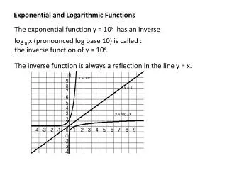
The inverse of y = 2x is x = 2y which is a reflection in the line y = x
Recall also x = 2y log2x = y Let’s draw the graph of y = log2x
This means that y = logax is the inverse of y = ax On your GC, draw the graphs of y = log2x log4x log10x Recall log2x = You can write y = and this will draw all three graphs at once
Using Graphmatica, let’s look at the graph of y = 4x and its derivative y = 3x and its derivative y = 2x and its derivative y = 2.5x and its derivative
y = 4x and its derivative y = 3x and its derivative y = 2x and its derivative y = 2.5x and its derivative Note where the derivative function is in relation to the function – in the first 2 cases, the derivative function is above the function and in the second two cases, it is below the function. Question: Is there a value such that the derivative function is exactly the same as the function?
This value is called e (the Euler number) e ≈ 2.71828…. y = ex dy= ex dx
y = ln(x) dy = 1 • dx x y = ln(kx) dy = 1 dx x Reason y = ln(kx) y = ln(u) where u = kx
Exercise New Q Page 79 Set 3.4 No. 1(a,b,c,e,f,h,i), 3(a-f), 4a Handout Sheet 244 – 281, 428-458 FM Page 459 Set 19.11 1,4,5-9
Solution of equations involving indices Model: Solve (a) 4e2x = 30 (b) 23x+1 = 40 • 4e2x = 30 (b) 23x+1 = 40 e2x = 7.5 3x + 1= log240 2x = ln 7.5 3x + 1 = (log 40)/(log 2) x = ½ ln 7.5 3x = (log 40)/(log 2)-1 x = 1.007 (3dp) x = ⅓ [ (log 40)/(log 2)-1 ] x = 1.441 (3dp)
Exercise New Q Page 83 Set 3.6
General Form of Exponential Graphs y = ex y = e-x Exponential graphs have a horizontal asymptote y = -e-x y = -ex
y=2 y = ex+2 y=1 y = ex+1 y = ex
Exponential graphs have a horizontal asymptote y=e3x y=ex y=e2x
Model: Determine a possible equation to describe the graph below: Use y=aebx + c 1. y=aebx -2 (1/2 , 3e-2) 2. When x=0, y=1 1 = aebx0 – 2 1 = a – 2 3 = a y = 3ebx -2 3. Using (1/2 , 3e-2) 3e-2 = 3e(b ½) – 2 3e = 3e(b ½) e = eb/2 b = 2 y = 3e2x – 2
Exercise New Q Page 102 Set 3.9 No. 1
General Form of Log Graphs y = ln(x) y = ln(-x) Logarithmic graphs have a vertical asymptote y = -ln(-x) y = -ln(x)
y=ln(x-1) y=ln(x) y=ln(x-2)
y=ln[-(x-1)] y=ln[-(x-2)] y=ln[-(x)]
(4,1) (3+e-1/2, 0) y = 2ln(x-3)+1