Download
1 / 22
220 likes | 334 Views
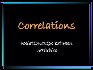
Correlations. Renan Levine POL 242 July 12, 2006. Association. :. Today: Correlations. Correlation is a measure of a relationship between variables. Measured with a coefficient [Pearson’s r ] that ranges from -1 to 1. Measure strength of relationship of interval or ratio variables

E N D
Correlations Renan Levine POL 242 July 12, 2006
Today: Correlations • Correlation is a measure of a relationship between variables. Measured with a coefficient [Pearson’s r] that ranges from -1 to 1. • Measure strength of relationship of interval or ratio variables • r = Σ(Zx * Zy)/n – 1 • Zx=Z scores for X variable and Z scores for Y variable. Sum the products and divide by number of paired cases minus one. • How to calculate Z scores can be found on-line.
Correlation r • Absolute values closer to 0 indicate that there is little or no linear relationship. • Generally, 0.2-0.4 is weak, 0.4-0.6 is okay, 0.6 or higher is strong. • If correlation is very high, then its probably something related that you might considering indexing or choosing just one variable. • The closer the coefficient is to the absolute value of 1 the stronger the relationship between the variables being correlated.
Positive Relationship • If two variables are related positively or directly • r > 0 • Variables “track together” – high values on Variable X are associated with high values on Variable Y. • Low values on X associated with low values.
Example Robert D. Putnam; Robert Leonardi; Raffaella Y. Nanetti; Franco Pavoncello. “Explaining Institutional Success: The Case of Italian Regional Government.” The American Political Science Review 77:1 (Mar. 1983), pp. 55-74 More fun examples: http://www.nationmaster.com/correlations/eco_gdp-economy-gdp-nominal
Example II r = 0.84
Negative or Inverse Relationship • Variables can be inversely or negatively related • High values of X are associated with low values of Y.
Example – Negative / Inverse r = -0.68 Time/SRBI: Oct 3-6, ‘08 red= Republicans, blue=Democrats, grey diamonds=Independents
Data • You need interval-level data. • You will find many interval-level variables in: • Countries / World • Provinces • Election studies (feeling thermometers, odds of party entering government, etc) • You can often use the index you created as an interval-level variable.
Compare Lots more noise here. Typical of public opinion data. Most points close to a line.
Differences between Public Opinion and Aggregate Data • Although it is not uncommon to have one/some outliers in aggregate data, public opinion data tends to be “noisy”. • Feeling thermometer example: • Many respondents gave both candidates a 50; • Quite a few respondents liked both candidates • Even though most who liked McCain disliked Obama • A high Pearson’s r for public opinion data may be low for an association in aggregate data.
Very Strong or Worrisome?? • Public Opinion: above |0.40| • Aggregate: above |0.80| • But these are just guidelines. It depends on how good the data is: • Lots of variation in data • Large scale (10, 20, 100 pts – like prediction odds, physicians per 100,000 people, feeling thermometer scales) • Number of observations (N) • Provinces dataset is small
Outstanding or the same? • You either have an outstanding relationship OR the variables may be measuring the same idea. • Ex. unemployment and GDP both measure economic health • Ex. Feeling thermometer Barack Obama and feeling thermometer for Joe Biden both measure attitudes towards the Democratic ticket • Also inverse relationship • Example above: Obama and McCain feeling thermometers – different sides of the same coin, as both seem to measure partisanship.
Use Yo’ Brain • Computer cannot tell you if it’s a good, strong relationship or two measures looking at the same thing. • Need to understand what each variable is measuring • Same thought process about the index creation. • Use your knowledge of world and theory to decide whether two variables measure the same thing or two different things. • Example (above): Putnam’s relationship between civic culture and government performance. • Failed states survey - appears that the higher an indicator value, the worse off the country in that particular field. • http://www.fundforpeace.org/web/index.php?option=com_content&task=view&id=99&Itemid=140
Flip side • Relationship you expect is strong is surprisingly not ?!?!? • Make certain both variables are interval • Double check that you cleaned up data • Missing values are missing • Next week: there may be the need to qualify the relationship as some sub-group of the data is not like the others and those need to be identified. • Think about relationship – maybe its not linear, so that relationship is only present for part of range.
Usefulness • Quick, easy way to look at several variables to see if they are related. • With strong association, you can begin to think about predicting values of Y based on a value of X. • Ex. Positive correlation – you know a high value of X is associated with a high value of Y!
Webstats Output - - Correlation Coefficients - - Q375A1 Q305 Q375A3 Q1005Q375A1 1.0000 .2916 .5320 -.3163 ( 686) ( 666) ( 667) ( 672) P= . P= .000 P= .000 P= .000Q305 .2916 1.0000 .2679 -.1272 ( 666) ( 2776) ( 660) ( 2721) P= .000 P= . P= .000 P= .000Q375A3 .5320 .2679 1.0000 -.2020 ( 667) ( 660) ( 682) ( 666) P= .000 P= .000 P= . P= .000Q1005 -.3163 -.1272 -.2020 1.0000 ( 672) ( 2721) ( 666) ( 3181) P= .000 P= .000 P= .000 P= . N Coefficients (Pearson’s r)
Significance? • Webstats will tell you whether or not the correlation coefficient is significant. • Remember that this is just telling you whether the relationship may be due to chance. • Not the strength of the relationship • Almost unheard of to have a strong relationship that is insignificant when using survey data. • So, don’t spend any time discussing significance.
What if non-interval/non-ratio? • Usually more appropriate to use the other measures of association. • Webstats will perform a correlation. Be ready for results to be less strong • Program may report (instead of Pearson’s r): • Spearman: ordinal x ordinal • Point-biserial: one interval/ratio, one dichotomous • Phi: two dichotomous variables • All interpreted the same way