Download
1 / 23
230 likes | 396 Views
Ice models vs. flasher data. Dima Chirkin, UW-Madison. History of SPICE model evolution 11/19/09 SPICE (also known as SPICE1): first version seeded with AHA as initial solution AHA is used for extrapolation above and below the detector

E N D
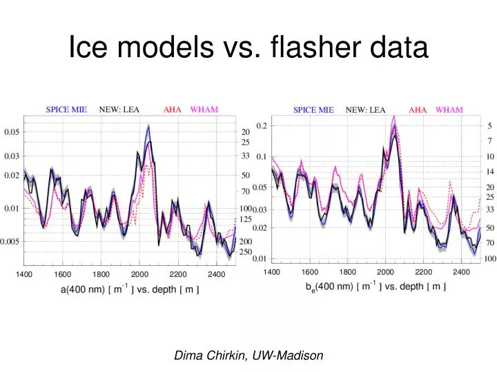
Ice models vs. flasher data Dima Chirkin, UW-Madison
History of SPICE model evolution 11/19/09 SPICE (also known as SPICE1): first version seeded with AHA as initial solution AHA is used for extrapolation above and below the detector relies on AHA for correlation relation between be(400) and adust(400). 02/01/10 SPICE2: fixed the hdh bug (see ppc readme file) seeded with bulk ice as initial solution dust logger and EDML data is used for extrapolation dust logger data is used to extend in x and y, taking into account layer tilt. 02/17/10 SPICE2+: fixed the "x*y" option hit counting in ppc be(400) vs. adust(400) relation is determined with a global fit to arrival time distributions. 04/28/10 SPICE2x: improved charge extraction in data: improved merging of the FADC and ATWD charges implemented saturation correction fixed the alternating ATWD bug updated DOM radius 17.8 --> 16.51 cm (cosmetic change: modifies only the meaning of py) fixed the DOM angular sensitivity curve (removed upturn at cos(theta)=-1). 06/09/10 SPICE2y: Fixed code determining the closest DOMs to the current layer (when using tilted ice) Iterations (after timing fits) are combined (improving description in the dust layer) Randomized the simulation based on system time (with us resolution). 07/23/10 SPICEMie: Much improved treatment of oversized DOMs in ppc Fits scattering function to a linear combination of HG and SAM functions, using higher g=0.9 Perform a global fit for py, overall time offset, scattering and absorption correlation coefficients Tilt map is estimated with respect to (0, 0) in IceCube coordinates (simplifies use with photonics). 04/16/12 SPICE Lea: Improved data processing with the new feature extraction Improved likelihood description and optimized binning Introduced and fitted ice anisotropy effect SPICE1: Relies on AHA as a first guess, and for correlation between be and adust. SPICE2: Adds extrapolation with dust logger and EDML, ice tilt map from Ryan SPICE2+: Use full arrival time distributions, full fit for both be and adust. SPICE Mie: Fit for toff and shape of the scattering function SPICE le-a: New NNLS-based feature extraction. Fitted ice anisotropy
Describing the data Ice model must describe the data to which it was fit, Ice model is built using the calibration in-situ light flasher data ice model must describe the flasher data1. Here I quantify the (dis)agreement with a width of the distribution of the charge ratio qsimulation/qdata for all pairs of emitters and receivers in a flasher data set. To reduce exertion I will only discuss this one parameter in this talk. 1) From Sarah Bouckoms SPE flasher study: the qualitative conclusions are the same, whether using low-light or high-intensity flasher light.
SPICE 1 threshold: > 0, 1, 10, 100, 400 p.e. 29.2%
SPICE Mie threshold: > 0, 1, 10, 100, 400 p.e. 27.7%
SPICE le-a threshold: > 0, 1, 10, 100, 400 p.e. 20.0%
AHA (fixed ppc table) threshold: > 0, 1, 10, 100, 400 p.e. 55.2%
WHAM threshold: > 0, 1, 10, 100, 400 p.e. 42.4%
Can we resolve ice anisotropy? N E Ice flow direction 41o NW C130-Skyway 8% more scattering 36o NW
SPICE 1 YES
SPICE Mie YES
SPICE le-a Resolved!
AHA (fixed ppc table) NO
WHAM NO
Can we resolve ice anisotropy? • SPICE 1: YES • SPICE Mie: YES • SPICE Lea: Resolved! • AHA: NO • WHAM: NO • Why not? • the data/simulation agreement is too poor • simulation prediction drops with distance too fast • this is average behavior! • So, not only the depth dependence is wrong, but also the relationship of absorption vs. scattering is wrong!
Conclusions Ice model error in description of the light deposition in the range of 125-250 meters away from the emitters: SPICE 1: 29.2% SPICE Mie: 27.7% SPICE Lea: 20.0% AHA: 55.2% WHAM: 42.4% SPICE1 provides a much better description than WHAM. SPICE Lea dramatically improves description of charge deposition.
Well, what about timing? See full collection of plots at http://icecube.wisc.edu/~dima/work/IceCube-ftp/ppc/lea/.