Download
1 / 19
190 likes | 242 Views
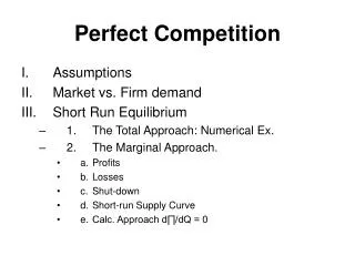
CHAPTER. 9. Perfect Competition. DEFINITION AND CHARACTERISTICS OF A PERFECTLY COMPETITIVE MARKET. Definition A market in which there are many buyers and sellers, the products are homogeneous and sellers can easily enter and exit from the market. Characteristics

E N D
MICROECONOMICS CHAPTER 9 Perfect Competition
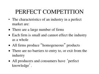
MICROECONOMICS DEFINITION AND CHARACTERISTICS OF A PERFECTLY COMPETITIVE MARKET Definition A market in which there are many buyers and sellers, the products are homogeneous and sellers can easily enter and exit from the market. • Characteristics • Large number of buyers and sellers – firms are price takers.
DEFINITION AND CHARACTERISTICS OF A PERFECTLY COMPETITIVE MARKET (CON’T) • Homogenous or standardized product – the buyers do not differentiate the products of one seller to another seller. • Free of entry and exit into the market. • Role of non-price competition is insignificant. • Perfect knowledge of the market – all the sellers and buyers in perfect competition market will have perfect knowledge of that market.
The price is determined by the intersection of the market supply curve and the market demand curve. Since firms are price takers, they face a horizontal demand curve. Demand curve in perfect competition is horizontal or perfectly elastic. Therefore, Price = MR = AR. Price Price SS RM10 P = MR = AR RM10 DD Quantity Q* Quantity Market Firm PRICE DETERMINATION IN A PERFECTLY COMPETITIVE FIRM
Using Table: Profit maximization is determined by scanning through the profit at each level, and the level which gives the highest profit is the profit maximizing output. (1) Quantity (per kg per dAy) (2) Price (per kg per dAy) 5) Profit/ Lloss (3) Total Revenue (TR) (4) Total Cost (TC) 0 10 20 30 40 50 60 70 10 10 10 10 10 10 10 10 0 100 200 300 400 500 600 700 60 140 210 290 390 500 630 800 -60 -40 -10 10 10 0 -30 -100 PROFIT MAXIMIZATION IN A PERFECTLY COMPETITIVE FIRM 1. Using Total approach TOTAL REVENUE – TOTAL COST APPROACH
TR, TC TC TR Highest vertical difference Quantity 40 PROFIT MAXIMIZATION IN A PERFECTLY COMPETITIVE FIRM Using Graph: TR curve is a straight line through the origin. The maximum profit is where the vertical difference is the highest.
(1) Quantity (per kg per day) (2) Price (per kg per day) (3) Total Revenue (TR) (4) Marginal Revenue (MR) (5) Total Cost (TC) (6) Marginal Cost (TC) (7) Profit/ Lloss Using Table: The profit maximizing output level is obtained following the MR = MC rule. 0 10 20 30 40 50 60 70 - 8 7 8 10 11 13 17 -60 -40 -10 10 10 0 -30 -100 0 100 200 300 400 500 600 700 10 10 10 10 10 10 10 10 - 10 10 10 10 10 10 10 60 140 210 290 390 500 630 800 PROFIT MAXIMIZATION IN A PERFECTLY COMPETITIVE FIRM 2. Using Marginal approach MARGINAL REVENUE – MARGINAL COST APPROACH
MR, MC MC RM10 MR Quantity 40 PROFIT MAXIMIZATION IN A PERFECTLY COMPETITIVE FIRM Using Graph: TR curve is a straight line through the origin. The maximum profit is where the vertical difference is the highest.
PROFIT MAXIMIZATION USING THE EQUATION METHOD The demand function for a product sold by a perfect competitor is given as QD = 20 – P and the marginal cost is MC = −10 + 3Q. Calculate profit maximizing price and quantity.
PROFIT MAXIMIZATION USING THE EQUATION METHOD (CON’T) Solution For profit maximization to take place, we use the MR = MC rule. Firstly, we need to derive the demand curve. Given Q = 20 − P P = 20 − Q MR = 20 − Q (since in perfect competitive firm, P = MR = AR)
PROFIT MAXIMIZATION USING THE EQUATION METHOD (CON’T) MR = MC 20 − Q = −10 + 3Q 4Q = 30 Q = 7.5 Substitute Q = 7.5 into P = 20 − Q P = 20 − 7.5 P = 12.5
Price (RM) AC e 20 P1 = MR1 = AR1 AVC d P = MR = AR 10 The portion of marginal cost curve which lies above the average variable cost curve is the firm’s supply curve. c P2 = MR2 = AR2 b P3 = MR3 = AR3 5 P4 = MR4 = AR4 a Supply curve of a competitive firm is the upward portion of MC above minimum of AVC as shown by points b, c, d and e. 60 Quantity 40 SHORT-RUN SUPPLY CURVE The figure shows the AC, AVC and MC. There are five different market prices. The horizontal demand curve at each price is shown. MC Point a is not considered a supply curve since at any point below the minimum of AVC, the firm would shut down its operation and the quantity supplied would be zero.
MC ATC The marginal cost curve intersects the demand curve at point B. A competitive firm maximizes its profit when MR = MC. PROFIT The profit maximizing price and output is P* and Q*. P = MR = AR At output Q* respectively the firm earns economic profit or supernormal profit equal to the area shaded. PROFIT MAXIMIZATION IN THE SHORT RUN A competitive firm earns economic profit Price (RM) The firm’s demand curve is horizontal at the price of RM20 where AR = MR. B P* 20 Economic profit or supernormal profit is the profit earned by a competitive firm when TR>TC. Q* Quantity
MC Price (RM) ATC B P* P = MR = AR 20 Q* Quantity PROFIT MAXIMIZATION IN THE SHORT RUN (CON’T) A competitive firm at breakeven Normal profit or breakeven profit is necessary for a firm to stay in business (TR =TC). At output Q*, the firm is at breakeven and earns normal profit. The profit maximizing price and output is P* and Q*, respectively. The firm’s demand curve is horizontal at the price of RM20 where AR = MR. The marginal cost curve intersects the demand curve at point B. A competitive firm maximizes its profit when MR = MC.
The firm’s demand curve is horizontal at the price of RM20 where AR = MR. MC Price (RM) The marginal cost curve intersects the demand curve at point B. A competitive firm maximizes its profit when MR = MC. ATC The profit maximizing price and output is P* and Q* respectively. B P* 20 P = MR = AR LOSSES At output Q*, the firm suffers economic losses or subnormal profit equal to the area shaded. Quantity Q* PROFIT MAXIMIZATION IN THE SHORT RUN (CON’T) A competitive firm suffers economic losses Economic losses or subnormal profit is the losses incurred by a competitive firm when TR<TC.
A firm can continue production until the price is equal to minimum average variable cost (AVC). AVC PROFIT MAXIMIZATION IN THE SHORT RUN (CON’T) SHUT DOWN PRICE A firm will continue its operations even if it suffers losses. MC Price (RM) At the price of RM5, the losses incurred by the firm is equal to the fixed cost. ATC B P = MR = AR If price falls below RM5, the firm would incur more operating losses than fixed cost and the firm must shut down. 20 TOTAL FIXED COST LOSSES 5 Shut down point is at the point where the price equals to minimum AVC. Q* Quantity
PROFIT MAXIMIZATION IN THE SHORT RUN(CON’T) EFFECT OF ENTRY Price is determined by the intersection of the market supply curve and the market demand curve. Firms that earn supernormal profits in short run will only be able to earn normal or zero profits in long run due to entry of newcomers. Price (RM) Price (RM) The economic profit attracts newcomers to the industry. As a result, many firms will enter the market and this will lead to an increase in supply. MC AC SS 20 SS1 P = MR = AR 20 15 PROFIT 15 P1 = MR1 = AR1 DD Quantity Quantity 60 Q* Supply curve will shift to the right and equilibrium market price will fall to RM15. The competitive firm sells 60 kg of chicken and earns an economic profit shown by the shaded area. Market Firm
PROFIT MAXIMIZATION IN THE LONG RUN EFFECT OF EXIT Supply curve will shift to left and equilibrium market price will rise to RM15 Firms that suffer losses in short run can still continue their operation. As in long run they are able to earn normal or zero profits due to exit of the firms. The losses in short run forces those sellers who cannot cover their AVC or TVC to leave the market. As many firms exit the market, this will lead to a decrease in the market supply. The competitive firm sells 60 kg of chicken and suffers losses shown by the shaded area. Price (RM) Price (RM) MC AC SS 10 SS1 P = MR = AR 20 15 LOSSES 15 P1 = MR1 = AR1 DD Quantity Quantity Market Firm 60 Q*