Download

1 / 51
520 likes | 676 Views
What shapes galaxy SEDs?. What shapes galaxy SEDs?. Stars Dust Gas Key papers Kennicutt 1998; Worthey 1994; Bell & de Jong 2001; Condon 1992; Bell 2003; Calzetti 2001 Osterbrock’s book…. Orientation 1. Energy balance optical : IR is ~ 50:50 in massive galaxies (like the Milky Way)

E N D
What shapes galaxy SEDs? • Stars • Dust • Gas • Key papers • Kennicutt 1998; Worthey 1994; Bell & de Jong 2001; Condon 1992; Bell 2003; Calzetti 2001 • Osterbrock’s book…
Orientation 1 Energy balance optical : IR is ~ 50:50 in massive galaxies (like the Milky Way) Both optical and IR have combination of ~black body + narrower features Sources: Stars Dust Gas
Orientation 2 Near-infrared dominated by long-lived stars Thermal infrared dust-reprocessed light from young stars 21cm emission from Neutral Hydrogen
1 Stars • Complex mix of stellar spectra • Flux at one wavelength: ∫∫∫f(M,Z,t) (t,Z) n(M) dM dZ dt • n(M) - the stellar IMF • (t,Z) - the star formation history • f(M,Z,t) - stellar library, complicated…
1.1 The stellar IMF n(M) • Critical assumption • Universally-applicable stellar IMF • In what follows choose Kroupa (2001) or Chabrier (2003) IMF
1.2 Star formation history (t,Z) • Often the parameter of interest • Points to note: • Z expected to evolve - in most cases it is ~OK to neglect Z evolution and simply solve for/assume <Z> • Because young stars so bright • What one assumes about recent SFH is important • What one assumes about ancient SFH less so…
1.3 Stellar library f(M,Z,t) • Straight sum of luminosities • Young main sequence very bright • blue • Post-main sequence short-lived but bright • Often red • Low-mass stars (those that make up the bulk of the mass) very faint • ‘Luminosity-weighted’ • Skews one’s view towards young/post-MS stars…
Color-Temperature • Hot stars (primarily young) are blue • Cooler stars are red • Giants (rare,bright) • Main sequence (common,faint)
What does this look like? SFR * IMF * flux for individual stars (before it’s integrated over all stars…) ~ the integrand… Left: “Painted” young to old Right: “Painted” old to young Top panels: Increasing SFR to emphasize recent star formation Bottom panels: constant SFR. Synthetic CMDs created by D. Weisz using Dolphin’s codes
1.4 Results 1.4.1 dependence of contributions (Worthey et al. 1994)
1.4.2 Distinctive / important features • 4000 angstrom break • 1.6um bump (from a minimum in H- opacity; much of the opacity from stars is from H-)… • Most important absorption lines • Balmer lines, metal lines Sawicki 2002
1.4.3 Age-metallicity degeneracy • The age-metallicity degeneracy: • Young, metal-rich populations strongly resemble old, metal-poor populations. [Fe/H]=-0.4 1.5 Gyr 1.0 Gyr 15 Gyr 7 Gyr Age=6 Gyr ,[Fe/H]=0.2 Age=12Gyr,[Fe/H]=0.0 2.0 Gyr [Fe/H]=-2.25 Models: Bruzual & Charlot (2003) Models: Sanchez-Blazquez (Ph.D. thesis); Vazdekis et al. 2005 (in prep)
1.4.3 a Some discrimination • Long wavelength baseline • MSTO vs. giant-sensitive line indices Trager 2000
1.4.4 Stellar masses • Age-metallicity degeneracy can work for us… • Stellar M/Ls close to unique function of SED shape • Cheap estimation of stellar masses. Bell et al. 2003
1.4.4.1 Normalisation : stellar IMF • Normalisation depends on stellar IMF • Salpeter IMF • too much mass in low-mass stars • Chabrier / Kroupa 2001 OK…
1.4.4.2 Stellar masses • Assumption - universal IMF • Methods • SED fitting Spectrum fitting • Comparison with dynamics: ~0.1 dex scatter Recent bursts de Jong & Bell, 2002- 2009; in prep. Comparing M* for SDSS galaxies SED vs. spectrum Me vs. Panter SED-based
1.4.4.3 Example stellar M/L calibns Kroupa / Chabrier -- actually -0.1 dex (Borch et al. 2006)
Summary I : stars • Almost all energy from galaxies is from stars (direct or reprocessed) • Emergent spectrum is triple integral • IMF (often assume universal),SFH, stellar library • Straight sum of luminosities • Weighted towards young, post-MS stars • Age/metallicity degeneracy • Some useful features comparing MSTO/Giants • Stellar masses • Uses age/met degeneracy - colors/spectra • Good to 30% in good conditions
1.5 - an in-depth application of stars - resolved stellar populationanalysis Thanks to Jason Harris and Evan Skillman
Synthetic CMDs created by D. Weisz using Dolphin’s codes Left: “Painted” young to old Right: “Painted” old to young Top panels: Increasing SFR to emphasize recent star formation Bottom panels: constant SFR.
DDO 165 in the M81 group Complete Star Formation History Note resolution at recent times better than ancient pops. Key result : star formation histories of dwarf galaxies tend to be bursty…
A Key Result…. • Dolphin et al. 2005 (on astroph) • Irregulars --> Spheroidals through gas loss alone (I.e., SFHs at ancient times v. similar)
Results de Jong et al. 2007 Stellar truncations also in old populations; not *just* star formation thresholds…
Summary II : CMDs • Color-magnitude diagrams • Very powerful • If get to main sequence turn off for old stars • Star formation history • Resolution good for recent star formation, worse for ancient times • Some chemical evolution history (better if have a few red giant spectra, helps a lot) • If you don’t get to main sequence turn off • Some SFH information remains but tricky to do well because it’s all post-main sequence based • Method • Match distribution of stars in color-magnitude space, maximise likelihood (e.g., minimise chi^2) • Key result : star formation histories of dwarf galaxies have considerable bursts • Key result : star formation histories of gas-rich and gas-poor dwarfs different only in last couple Gyr - gas removal only difference?
Dust attenuation and emission Thanks to Brent Groves
2. Dust • Dust absorbs and scatters UV/optical light, energy heats grains and they emit in the thermal IR • 2.1 - emission from dust grains • 2.2 - extinction/attenuation
Spectrum Stolen from a talk by Brent Groves
2.1.1 Dust - key concepts • Absorption of UV/optical photons (1/2 to 2/3 of all energy absorbed + re-emitted) • Grains re-emit energy • Grain size distribution • PAHs - various benzene-style modes (very small, big molecules, band struc) • Very small grains - transient heating • Larger grains - eqm heating
2.1.2 Dust - key concepts II • Thermal equilibrium • 4 r2 T4 = (L*/ 4d2) r2 (1-A) • T4 = (L*/ 4d2) (1-A)/4 • Independent of dust grain size • Challenge - name 3 or 4 situations when you’ve seen the consequences of this before… Emission Local radn density Absorption
2.1.2.1 Small grains not in equilibrium • Smallest grains • small cross-section • hence low photon heating rate • However, small grains also • low specific heat • one photon causes large increase in Temperature Credit: Brent Groves
2.1.3 Ingredients of a dust model • Grain size distribution • Solve for temperature distribution given radiation field • Paint on black bodies of that temperature • Add PAH features (usually by hand!) • Radiation field from stellar models + geometry • Dust geometry critical - controls how much energy absorbed and temp of emitting dust. • Definition : Photodissociation Region • All regions of ISM where FUV photons dominate physical/chemical processes
2.1.4 Case study: dust masses • Mass = flux * d2 / [dust cross section per unit mass * planck function (at a temperature T, at measured frequency)] • *highly* uncertain, need longest wavelengths possible and understand what fraction of dust is at which temperatures • Long wavelength cross section uncertain • End up with gas/dust of ~200-300 (Sodroski et al. 1994; Dunne et al. 2000)
Case study: dust masses • Mass = flux * d^2 / (dust cross section per unit mass * planck function(at a temperature T, at measured frequency) • *highly* uncertain, need longest wavelengths possible and understand what fraction of dust is at which temperatures • Long wavelength cross section uncertain • End up with gas/dust of ~200-300 (Sodroski et al. 1994; Dunne et al. 2000)
2.2 Extinction • Absorption and scattering • Thus, geometry is critical • Optically-thick distributions behave less intuitively Forward scattering Draine 2003
2.2.1 Extinction • Extinction curve is variable, esp in FUV • Argues shocks / radiation field from nearby star formation - Gordon et al. 2003 Cartledge et al. 2005
2.2.2 Attenuation vs. extinction • Excinction curve = for a star, absorption and scattering • Attenuation curve = for a galaxy, a complicated mix of absorption, scattering and geometry • See e.g., Witt & Gordon 2000 for a discussion…
2.2.3 Dust attenuation models • Have to track properly • Monte Carlo techniques (Karl Gordon, Roelof de Jong, others) • Charlot & Fall, Calzetti (2001) • Attenuation(stars) ~ 0.44 x attenuation(gas) • Motivation - escaping birth cloud
2.2.4 Simple toy model consideration • Optical depth gas surface density * metallicity • Motivation - dust/gas metallicity • Total dust column gas column Bell 2003