Download
1 / 51
510 likes | 655 Views
Probabilistic Paths and Centrality in Time. Joseph J. Pfeiffer, III Jennifer Neville. a. b. c. d. e. f. a. b. Betweenness Centrality. c. d. e. f. Aggregate. Time 1. Time 2. Time 3. Time 4. Time 5. Time Varying Graphs. a. b. a. b. a. b. a. b. a. b. a. b. =. c.

E N D
Probabilistic Paths and Centrality in Time Joseph J. Pfeiffer, III Jennifer Neville
a b c d e f
a b Betweenness Centrality c d e f
Aggregate Time 1 Time 2 Time 3 Time 4 Time 5 Time Varying Graphs a b a b a b a b a b a b = c d c d c d c d c d c d e f e f e f e f e f e f
Aggregate Time 1 Time 2 Time 3 Time 4 Time 5 Time Varying Graphs a b a b a b a b a b a b = c d c d c d c d c d c d e f e f e f e f e f e f Represent Current Graph
Aggregate Time 1 Time 2 Time 3 Time 4 Time 5 Time Varying Graphs a b a b a b a b a b a b = c d c d c d c d c d c d e f e f e f e f e f e f Represent Current Graph Betweenness Centrality
Aggregate Time 1 Time 2 Time 3 Time 4 Time 5 Time Varying Graphs a b a b a b a b a b a b = c d c d c d c d c d c d e f e f e f e f e f e f Represent Current Graph Betweenness Centrality
Aggregate Time 1 Time 2 Time 3 Time 4 Time 5 Time Varying Graphs a b a b a b a b a b a b = c d c d c d c d c d c d e f e f e f e f e f e f Messages are irregular – large changes in metric values between slices
Related Work • Betweenness centrality throughtime (Tang et al. SNS ’10) • Vector clocks for determining edges with minimum time-delays (Kossinetset al. KDD ’08) • Finding patterns of communication that occur in time intervals (Lahiri & Berger-Wolf, ICDM ’08)
a b Time 1 Time 2 Time 3 Time 4 Time 5 a b a b a b a b a b c d c d c d c d c d c d e f e f e f e f e f e f
a b Time 1 Time 2 Time 3 Time 4 Time 5 .65 Probabilistic Graphs a b a b a b a b a b .95 .8 c d c d c d c d c d .8 c d e f e f e f e f e f .95 .8 .65 .8 .8 e f
a b Time 1 Time 2 Time 3 Time 4 Time 5 .65 Probabilistic Shortest Paths a b a b a b a b a b .95 .8 c d c d c d c d c d .8 c d e f e f e f e f e f .95 .8 .65 .8 .8 e f
a b Time 1 Time 2 Time 3 Time 4 Time 5 .65 Probabilistic Shortest Paths a b a b a b a b a b .95 .8 c d c d c d c d c d .8 c d e f e f e f e f e f .95 .8 .65 .8 .8 a-c-b: .95*.65 = 0.61 e f
a b Time 1 Time 2 Time 3 Time 4 Time 5 .65 Probabilistic Shortest Paths a b a b a b a b a b .95 .8 c d c d c d c d c d .8 c d e f e f e f e f e f .95 .8 .65 .8 .8 a-c-b: .95*.65 = 0.61 a-d-b: .80*.80 = 0.64 e f
a b Time 1 Time 2 Time 3 Time 4 Time 5 .65 Probabilistic Shortest Paths a b a b a b a b a b .95 .8 c d c d c d c d c d .8 c d e f e f e f e f e f .95 .8 .65 .8 .8 a-c-b: .95*.65 = 0.61 a-d-b: .80*.80 = 0.64 a-c-d-b: .95*.95*.80 = 0.72 e f
a b Time 1 Time 2 Time 3 Time 4 Time 5 .65 Probabilistic Shortest Paths a b a b a b a b a b .95 .8 c d c d c d c d c d .8 c d e f e f e f e f e f .95 .8 .65 .8 .8 a-c-b: .95*.65 = 0.61 a-d-b: .80*.80 = 0.64 a-c-d-b: .95*.95*.80 = 0.72 (1-0.61)*(1-.64)*0.722 e f
a b Time 1 Time 2 Time 3 Time 4 Time 5 .65 Probabilistic Shortest Paths a b a b a b a b a b .95 .8 c d c d c d c d c d .8 c d e f e f e f e f e f .95 .8 .65 .8 .8 a-c-b: .95*.65 = 0.61 a-d-b: .80*.80 = 0.64 a-c-d-b: .95*.95*.80 = 0.72 (1-0.61)*(1-.64)*0.722 e f
a b Time 1 Time 2 Time 3 Time 4 Time 5 .65 Probabilistic Shortest Paths a b a b a b a b a b .95 .8 c d c d c d c d c d .8 c d e f e f e f e f e f .95 .8 .65 .8 .8 a-c-b: .95*.65 = 0.61 a-d-b: .80*.80 = 0.64 a-c-d-b: .95*.95*.80 = 0.72 (1-0.61)*(1-.64)*0.722 Shared Edges e f
a b Time 1 Time 2 Time 3 Time 4 Time 5 .65 Probabilistic Shortest Paths a b a b a b a b a b .95 .8 c d c d c d c d c d .8 c d e f e f e f e f e f .95 .8 .65 .8 .8 a-c-b: .95*.65 = 0.61 a-d-b: .80*.80 = 0.64 a-c-d-b: .95*.95*.80 = 0.72 (1-0.61)*(1-.64)*0.722 Shared Edges e f
a b Time 1 Time 2 Time 3 Time 4 Time 5 .65 Probabilistic Shortest Paths a b a b a b a b a b .95 .8 c d c d c d c d c d .8 c d e f e f e f e f e f .95 .8 .65 .8 .8 Intractable to Compute Exactly e f
a b Time 1 Time 2 Time 3 Time 4 Time 5 .65 Probabilistic Shortest Paths a b a b a b a b a b .95 .8 c d c d c d c d c d .8 c d Approximate with Sampling e f e f e f e f e f .95 .8 .65 .8 .8 Intractable to Compute Exactly e f
a b Time 1 Time 2 Time 3 Time 4 Time 5 .65 Probabilistic Shortest Paths a b a b a b a b a b .95 .8 c d c d c d c d c d .8 c d e f e f e f e f e f .95 .8 .65 .8 .8 Sample each edge independently e f
a b Time 1 Time 2 Time 3 Time 4 Time 5 .65 Probabilistic Shortest Paths a b a b a b a b a b .95 .8 c d c d c d c d c d .8 c d e f e f e f e f e f .95 .8 .65 .8 .8 Sample each edge independently Distribution of graphs e f
a b Time 1 Time 2 Time 3 Time 4 Time 5 .65 Probabilistic Shortest Paths a b a b a b a b a b .95 .8 c d c d c d c d c d .8 c d e f e f e f e f e f .95 .8 .65 .8 .8 Sample each edge independently Distribution of graphs Expected Betweenness Centrality e f
a b Time 1 Time 2 Time 3 Time 4 Time 5 .65 Most Likely Paths a b a b a b a b a b .95 .8 c d c d c d c d c d .8 c d e f e f e f e f e f .95 .8 .65 .8 .8 Most Likely Path e f
a b Time 1 Time 2 Time 3 Time 4 Time 5 .65 Most Likely Paths a b a b a b a b a b .95 .8 c d c d c d c d c d .8 c d e f e f e f e f e f .95 .8 .65 .8 .8 a-c-b: .95*.65 = 0.61 a-d-b: .80*.80 = 0.64 a-c-d-b: .95*.95*.80 = 0.72 e f
a b Time 1 Time 2 Time 3 Time 4 Time 5 .65 Most Likely Paths a b a b a b a b a b .95 .8 People with strong relationships are still unlikely to pass on all information… c d c d c d c d c d .8 c d e f e f e f e f e f .95 .8 .65 .8 .8 a-c-b: .95*.65 = 0.61 a-d-b: .80*.80 = 0.64 a-c-d-b: .95*.95*.80 = 0.72 e f
a b Time 1 Time 2 Time 3 Time 4 Time 5 .65 Most Likely Handicapped (MLH) Paths a b a b a b a b a b .95 .8 c d c d c d c d c d .8 c d e f e f e f e f e f .95 .8 .65 .8 .8 a-c-b: 0.61*β2 a-d-b: 0.64*β2 a-c-d-b: 0.72*β3 e f Transmission Probability
a b Time 1 Time 2 Time 3 Time 4 Time 5 .65 MLH Paths a b a b a b a b a b .95 .8 c d c d c d c d c d .8 c d e f e f e f e f e f .95 .8 .65 .8 .8 a-c-b: 0.61*.52= 0.15 a-d-b: 0.64*.52 = 0.16 a-c-d-b: 0.72*.53 = 0.09 e f Transmission Probability
a b Time 1 Time 2 Time 3 Time 4 Time 5 .65 MLH Paths a b a b a b a b a b .95 .8 c d c d c d c d c d .8 c d e f e f e f e f e f .95 .8 .65 .8 .8 a-c-b: 0.61*.52= 0.15 a-d-b: 0.64*.52 = 0.16 a-c-d-b: 0.72*.53 = 0.09 e f Transmission Probability
a b Time 1 Time 2 Time 3 Time 4 Time 5 .65 MLH Paths a b a b a b a b a b .95 .8 c d c d c d c d c d .8 c d e f e f e f e f e f .95 .8 .65 .8 .8 a-c-b: 0.61*.52= 0.15 a-d-b: 0.64*.52 = 0.16 a-c-d-b: 0.72*.53 = 0.09 e f TransmissionProbability Easy to Compute
a b Time 1 Time 2 Time 3 Time 4 Time 5 .65 MLH Paths a b a b a b a b a b .95 .8 Use MLH Paths for Betweenness Centrality c d c d c d c d c d .8 c d e f e f e f e f e f .95 .8 .65 .8 .8 a-c-b: 0.61*.52= 0.15 a-d-b: 0.64*.52 = 0.16 a-c-d-b: 0.72*.53 = 0.09 e f TransmissionProbability Easy to Compute
Link Probabilities: Relationship Strength 1 P(e) 0 Time
Link Probabilities: Relationship Strength 1 P(e) 0 Time Probability of no message contributing to relationship
Link Probabilities: Relationship Strength 1 = * P(e) 0 Time Probability of no message contributing to relationship
Link Probabilities: Relationship Strength 1 = - = * P(e) 0 Time Probability of no message contributing to relationship
Link Probabilities: Relationship Strength 1 = - = * P(e) Any Relationship Strength 0 Time Probability of no message contributing to relationship
Enron Emails • 151 Employees – 50,572 messages over 3 years • Known dates in time • 10,000x for Sampling Method • Time slice length was 2 weeks • Evaluated all metrics at end of every two weeks • Aggregate, Slice, Sampling, MLH Evaluation
Method Correlations and Sample Size Aggregate/Sampling Sampling Aggregate Slice/Sampling Slice Aggregate/Slice
Lay Lay Lay and Skilling Skilling Skilling Sampling MLH Lay Lay Skilling Skilling Slice Aggregate
Kitchen Kitchen Lavorato and Kitchen Lavorato Lavorato Sampling MLH Kitchen Lavorato Lavorato Kitchen Slice Aggregate
Shortest Paths on Unweighted Discrete Graphs are a special case of Most Likely Handicapped Paths
Discrete Probabilistic Shortest Paths and Most Probable Handicapped Paths 1
Discrete Probabilistic Shortest Paths and Most Probable Handicapped Paths 1 Length: 1 Probability: β
Discrete Probabilistic Shortest Paths and Most Probable Handicapped Paths … … 1 Length: n Probability: βn
Discrete Probabilistic Shortest Paths and Most Probable Handicapped Paths … … 1 Length: n n < n+1 Probability: βn βn > βn+1
Discrete Probabilistic Shortest Paths and Most Probable Handicapped Paths … … 1 Shortest Paths can be formulated as Most Probable Handicapped Paths Length: n n < n+1 Probability: βn βn > βn+1
MLH Paths: Modify Dijkstra’s. Rather than shortest path for expansion, choose most probable path. Computation MLH Betweenness Centrality: Modify Brandes’. Rather than longest path for backtracking, choose least probable path.
Conclusions Developed sampling approach Developed most probable paths formulation Incorporated inherent transmission uncertainty Evaluated on Enron email dataset Aggregate representations of time evolving graphs are unable to detect changes with the graph Slice samples of the graph have large variation from one slice to the next Future Work: Additional metrics, such as probabilistic clustering coefficient