Download
1 / 19
190 likes | 287 Views
Assessing the detection capability of the International Monitoring System infrasound network. David Green and David Bowers. AWE Blacknest. Assessing the detection capability of the International Monitoring System infrasound network. David Green and David Bowers. AWE Blacknest.

E N D
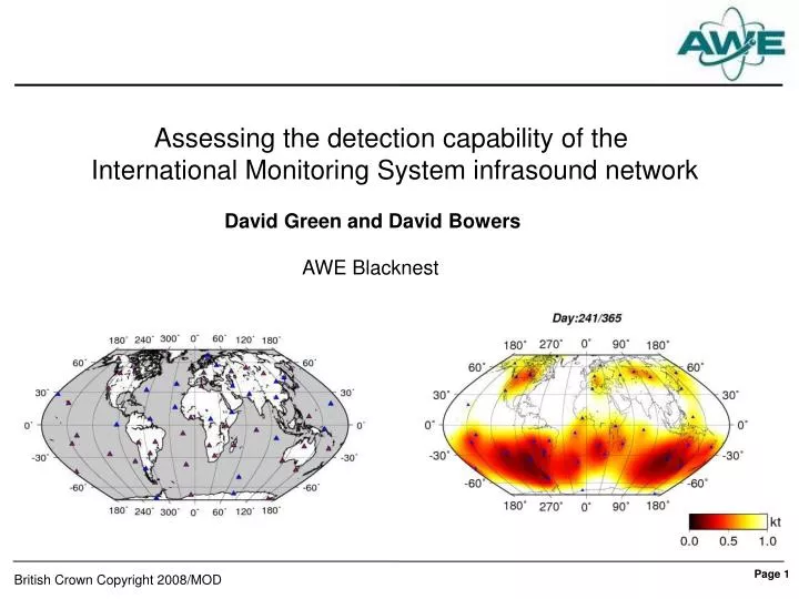
Assessing the detection capability of the International Monitoring System infrasound network David Green and David Bowers AWE Blacknest
Assessing the detection capability of the International Monitoring System infrasound network David Green and David Bowers AWE Blacknest Talk Outline 1. Previous Models - Stratospheric Wind 2. Extensions - Noise - Array Processing - Frequency Dependence 3. Results 4. Comparison to observed: Gerdec Explosions
( ) + Previous Work IMS infrasound network • 60 stations when complete ( ) • 37 arrays as of July 2007 • Previous models: • incorporate Yield vs. Amplitude • relationships • incorporate noise measurements • no wind incorporated (e.g., Clauter and Blandford, 1998, Stevens et al. 2002) (following Stevens et al. 2002)
Extended Model Components Amplitude dependence on: Array Processing Noise SNR enhancements 1. Yield (Bowman et. al, 2007) 2. Stratospheric Wind Conditions (Whitaker et al. 2003) Frequency Dependence (Noise Models and Yield Relationships) Network Completeness Detection Capability
The Model • Calculate the probability, Pijk, that a signal will be detected • at station i for an event k occurring at location j. • Assume that noise distribution is taken as log-normal (after e.g., Clauter and Blandford, 1998) • We define the detection threshold as the yield at which the probability of detecting an event • at two or more stations in the network exceeds 0.9. Pdetect = 1 − Pno detect − Pone detec Prob. of detection Probability of no detection across network Probability of detection at only one station across network
The Model Station reliability Uncertainities in signal and noise amplitude The probability that a signal will be detected at station i for an event k occurring at location j. The signal-to-noise level at which a detection can be made divided by signal-to-noise improvement from beamforming. The predicted signal-to-noise ratio at the station. (log10-log10) We use a single channel signal-to-noise ratio = 1 for the calculations shown.
Noise Models Used (Bowman et. al, 2007) • Used noise models from Bowman et. al, 2007 • An analysis of 39 stations (34 IMS) • - 44 months of data used • Figure to right shows median spectra (solid line) • and the 5th and 95th percentile spectra (dotted lines). • In our detection capability models we assume • time-independent, station-independent noise model Extending to time and location dependent models is a necessary future improvement (already implemented by Le Pichon et al, 2008).
Array Processing: Signal-to-Noise Improvements • A study of 6 events showed gains of between 0.7 and 1.1 x √n • (where n = no. of array elements) Beam • For all modelling, used value of 0.9√n Single Channel Signal Window Pre-event noise Neyshabur Train Explosion recorded at I31KZ (1 to 5 Hz) Christmas Island Bolide Recorded at I04AU (0.1 to 0.5Hz)
Frequency Dependence • At what frequency should we take our noise • estimates? or • Are different size sources going to be preferentially • observed at different frequencies? e.g., AFTAC Yield (Y) vs. Period (t) Equation • Can combine with the Whitaker Yield vs. Amplitude • relation to give Frequency vs. Amplitude relation. Source to Receiver range = 1000km
Adding the Stratospheric Wind: 59 Station Network 90% Detection Threshold (2 station) for the 59 station network. Noise from Bowman (2007) model, taken at 0.1Hz.
37 Station Network (Operational in 2007) 90% Detection Threshold (2 stat.) for the 37 station network. Noise from Bowman (2007) model, taken at 0.1Hz.
Comparing 37 and 59 Station Networks New York, 59 Stat. Nov. Zemlya, 59 Stat. • Incomplete network – • decrease detection prob. at specific locations • value dependent upon: • 1. the completeness of the regional network • 2. the influence of the dominant wind directions. Solid lines: with wind Nov. Zemlya, 37 Stat. New York, 37 Stat. Dotted lines: without wind
Location Capability : Influence of Stratospheric Wind With less wind - the angle of separation of the two detecting stations tends to be greater - the source to second receiver distance tends to be less High Wind No Wind Including wind – better detection capability, but apparently harder to locate source
Frequency Dependence Equivalent diagrams (Noise from AFTAC relation – indicates that the frequency at which the noise is taken from the Bowman et. al (2007) model is determined using the AFTAC yield vs. period relation). If noise variation with frequency is taken into account: - at low yields, achieve better global detections because of lower noise - if comparing with a single noise value (at 0.1Hz), only at the microbarom peak does the variable noise model perform less well than the frequency varying noise
Comparison with Gerdec Explosion Observations • Gerdec, Albania: • 2 large munitions dump explosions • 15th March 2008 • Highest SNR ~ 0.5Hz • Signal Power down to periods of ~30s Decreasing yield = Decreasing probability of single station detection. Dom. Signal Freq. Future IMS station Detecting IMS station Detecting non-IMS Non-detecting non-IMS
Comparison with Gerdec Explosion Observations Le Pichon et al., 2008 A more deterministic approach. Tons (TNT) (see Alexis’ talk) Green and Bowers, 2008 Adapted to incorporate: • ECMWF wind model • measured noise levels Uncertainties reduced to simulate deterministic approach. Two independent models. Converge to very similar results. Can compare and contrast techniques; underlying empirical models are identical
Model presented here is relatively simple in design; future improvements will include: • More accurate atmospheric parameterisation • Array-dependent wind noise • Improved understanding of 1. Yield vs. Pressure 2. Yield vs. Period Conclusions • Inclusion of stratospheric wind makes detection capability time dependent. • The completeness of the IMS network is vital for ensuring global coverage. • Inclusion of stratospheric wind tends to improve detection capability, • but hinders location capability for low yield explosions. • The frequencies of interest should be considered when calculating the network • detection capability.
References and Acknowledgements Bowman, J. R. et al. Infrasound Station Ambient Noise Estimates and Models: 2003-2006 Infrasound Technology Workshop, Tokyo, November 2007 Clauter, D. and Blandford, R. Capability Modelling of the Proposed International Monitoring System 60-Station Infrasonic Network. In Infrasound Workshop for CTBT, pages 215–225, Santa Fe, New Mexico, USA, August 25-28, 1997, (1998) LANL. LA-UR-98-56. Green, D. N., Assessing the detection capability of the International Monitoring System infrasound network AWE Report 629/08 (2008) (Available on request, dgreen@blacknest.gov.uk) Le Pichon, A. et al. Assessing the performance of the International Monitoring System infrasound network: Geographical coverage and temporal variabilities JGR – Atmospheres (in press, 2008) Stevens, J.L., Divnov, I.I., Adams, D.A., Murphy, J.R., and Bourchik, V.N. Constraints on Infrasound Scaling and Attenuation Relations from Soviet Explosion Data. Pageoph, 159, 1045–1062, (2002). Whitaker, R. W., Sondoval, T. D., and Mutschlecner, J. P. Recent Infrasound Analysis. In Proceedings of the 25th Annual Seismic Research Symposium in Tuscon, AZ, pages 646–654, (2003). Acknowledgements Fruitful discussions with Alexis Le Pichon, Lars Ceranna, Laslo Evers and Julien Vergoz helped improve this work, and highlighted possible avenues for future work. We thank Roger Bowman (SAIC) for providing us with the noise model across the IMS infrasound network.
From Probabilistic to Deterministic When comparing Le Pichon et al. (2008), and Green and Bowers (2008) By moving towards the deterministic model, we are saying: ‘We are confident that we can predict noise levels and stratospheric wind values’ and ‘We are confident that our empirical models provide the correct yield/pressure relationship’ Problem: how to correctly assess the uncertainties.