Download

1 / 63
630 likes | 805 Views
Adaptive Algorithms for Planar Convex Hull Problems. Yoshio Okamoto (Tokyo Institute of Technology, Japan) Joint work with Hee-Kap Ahn (Postech, Korea). Merge sort: motivating example. Split the input array into two smaller subarrays Recursively sort them

E N D
Adaptive Algorithms for Planar Convex Hull Problems Yoshio Okamoto (Tokyo Institute of Technology, Japan) Joint work with Hee-Kap Ahn (Postech, Korea)
Merge sort: motivating example • Split the input array into two smaller subarrays • Recursively sort them • Merge to obtain the whole sorted array • Running time: Θ(nlogn) for any n-elem array • Θ(nlogn) even if the input is already sorted
Adaptive sorting algorithms • A sorting algorithm is adaptive if it runs faster when the input is closer to being sorted Coined by Mehlhorn ’84 Surveyed by Estivill-Castro & Wood ’92 • Merge sort, Quick sort are not adaptive... Input scattered sorted slow fast Algorithm
How to measure the disorder • An inversion in an array A is a pair (i, j) s.t.i < j and A[i] > A[j] • # of inversions as a measure of disorder inversion
Adaptive sorting algorithms • There’re several adaptive sorting algorithmsrunning in O(n(1+log(1+k/n))) • n = # of elements in an input array • k = # of inversions in an input array Mehlhorn ’84 Mannila ’85 Levcopoulos & Petersson ’91 Levcopoulos & Petersson ’93 Elmasry ’02Elmasry & Fredman ’08 • The algorithms don’t need to know k
Optimality Running time O(n(1+log(1+k/n))) is optimal • Always k≤ n(n-1)/2Hence, O(n(1+log(1+k/n))) = O(nlogn) Optimal wrt n • There’s a lower bound Ω(n(1+log(1+k/n))) Guibas, McCreight, Plass & Roberts ’77Optimal wrt n & k • Much is known for adaptive sorting algorithms
Question • Sorting is a “1-dimensional” problem • How about 2-dimensional problems? Adaptive Computational Geometry
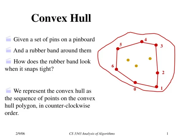
Case study: planar convex hull • Given a set of n pts in the plane (general pos’n) • Identify the convex hull in the clockwise order • Several O(nlogn) algorithms known, optimal Goal:to design an adaptive convex hull algorithm
Some issues to overcome • Need to specify the format of outputs so thatinputs and outputs can be compared wrt a measure of disorder • Need to define the disorder of inputs
In-place geometric algo’s inspire us • Input: an array of objects • Computation: rearrangement of the array • Output: an array of objects, too Brönnimann, Iacono, Katajainen, Morin, Morrison, Toussaint @LATIN’02, TCS ’04 Brönnimann, Chan, Chen @SoCG’04 Brönnimann, Chan @LATIN’04, CGTA’06 Bose, Maheshwari, Morin, Morrison, Smid, Vahrenhold @EWCG’04, CGTA’07 Vahrenhold @WADS’05, CGTA’07 Blunck, Vahrenhold @CIAC’06 Blunck, Vahrenhold @SWAT’06 Vahrenhold @IPL’07 Chan, Chen @SODA’08 Chan, Chen @CCCG’08 Chan, Chen @SoCG’09
See it as an ordering problem motivated by in-place geometric algo’s (Brönnimann et al. ’04) • Given an array of n planar points • Rearrange the array s.t. • The pts on the conv hull come first ordered by the clockwise order, and the leftmost pt top • The pts in the interior come next ordered by their x-coordinates 3 2 4 9 10 1 8 5 6 7
Rearranging the input array Input Output 6 3 9 1 10 7 5 8 2 4
Adaptivity in planar convex hulls • Input is an array • Output is an array,uniquely determined by the input,uniquely determines an order on the input points(if points are in sufficiently general position) • # inversions btw the input and the output:measure of disorder Input Output
Result Algorithm for the planar convex hull problem • running time: O(n(1+log(1+k))) • Algorithm doesn’t need to know k • k = 0 O(n(1+log(1+k))) = O(n) • Optimal wrt n • Not known to be optimal wrt n & k(Lower bound Ω(n(1+log(1+k/n))) from sorting) Remains as an open problem
You may think… • Unnatural that the pts in the interior need to be sorted by their x-coords Our second formulation 3 2 4 9 10 1 8 5 6 7
Second formulation equivalent to the setting by Brönnimann et al. ’04 • Given an array of n planar points • Rearrange the array s.t. • The pts on the conv hull come first ordered by the clockwise order, and the leftmost pt top • The pts in the interior come next, but in an arbitrary order 3 2 4 8 9 1 10 5 6 7
How to measure the disorder • Input is an array • Output is an array, not unique • Measure of disorder =min # inversions btw the input and the output over all possible (valid) outputs
Second result Lower bound for the second formulation • Any algorithm needs Ω(n log h) comparisons • h = # pts on the boundary of the conv hull • Remark: O(n log h)algorithm (Kirkpatrick-Seidel ’86) Therefore, no algorithm can make use of disorder
Summary of the results First formulation: interior pts need to be sorted • Algorithm w/ running time O(n(1+log(1+k))) Second formulation: int pts need not to be sorted • Lower bound of complexity Ω(n log h)
Other adaptive comp geom (1) Levcopoulos, Lingas & Mitchell (SWAT’02) • Convex hull of a polygonal chain • Parameter k: # self-intersections • UB: O(n log(k+2)) • LB: Ω(n log(k/n)) • Parameter χ: min size of a partition into simple paths • UB: O(n log(χ+2)) • LB: Ω(n log(χ+2))
Other adaptive comp geom (2) Barbay & Chen (CCCG’08) • Convex hull of convex polygons • Parameter δ: “certificate” size • Two polygons (n=total # vertices) • UB: O(δ log(n/δ)) • LB: Ω(δ log(n/δ)) • k polygons • UB: O(δk log(n/δk))
Features of our work • Looking at the most fundamental “convex hull of a point set” • Casting the problems into permutation problems(motivated by in-place algorithms) • Disorder is measured by the input and the output arrays
Summary of the results 1st formulation: interior pts need to be sorted • Algorithm w/ running time O(n(1+log(1+k))) 2nd formulation: interior pts need not to be sorted • Lower bound of complexity Ω(n log h) Now we concentrate on the first • Or we skip
Difficulty in algorithms design 1 • “Just looking at two points” cannot determine the correct pairwise order 6 3 9 1 10 7 5 8 2 4 Output
Difficulty in algorithms design 2 • A subproblem doesn’t inherit the correct order 6 3 9 1 10 7 5 8 2 4 Output
Algorithm: basic strategy • A la Kirkpatrick-Seidel’s algorithm (SICOMP’86) • Divide-and-conquer by median finding • Given a point set P, compute • the upper hull U(P), sorted by x-coords • the lower hull L(P), sorted by reverse x-coords • the interior I(P), sorted by x-coords • If k=0, the algorithm should run in O(n) time
Check if the input is already ok (1) • Identify the leftmost and the rightmost pts • O(n) time Input 6 3 9 1 10 7 5 8 2 4
Check if the input is already ok (2) • Identify the upper hull (concave chain) • O(n) time Input 6 3 9 1 10 7 5 8 2 4
Check if the input is already ok (3) • Identify the second leftmost pt on the lower hull • O(n) time Input 6 3 9 1 10 7 5 8 2 4
Check if the input is already ok (4) • Identify the lower hull (convex chain) • O(n) time Input 6 3 9 1 10 7 5 8 2 4
Check if the input is already ok (5) • Identify the pts in the interior (sorted) • O(n) time Input 6 3 9 1 10 7 5 8 2 4
Check if the input is already ok (6) • Check the pts in the interior are betweenthe upper & lower hulls • O(n) time Input 6 3 9 1 10 7 5 8 2 4
Algorithm outline: step 1 Input: a point set P (as an array) • Step 1: O(n) timeCheck if P is already ok, as already explained;Halt if P is ok
Algorithm outline: step 2 Input: a point set P (as an array) • Step 2: O(n) time (median finding, Blum et al. ’72)Find a bisector (wrt x-coords) of P • A = the pts on the left, B = the pts on the right
Algorithm outline: step 3 Input: a point set P (as an array) • Step 3: O(n) time (2-dim LP, Megiddo ’84)Find the upper & the lower tangents of P • Identify the points A(u), A(l), B(u), B(l)
Algorithm outline: step 4 Input: a point set P (as an array) • Step 4: O(n) timeConnect A(u), A(l) and B(u), B(l) • Partition into three parts L, M, R
Crucial properties: step 4 • The order of P inherits in L, M, R (overcoming the mentioned difficulties) • #inv(P) ≥ #inv(L) + #inv(M) + #inv(R)
Algorithm outline: step 5 Input: a point set P (as an array) • Step 5: Recursively run the algorithm on L & R • Obtain U(L), U(R), L(L), L(R), I(L), I(R)
Algorithm outline: step 6 Input: a point set P (as an array) • Step 6: Adaptively sort the points in M
Algorithm outline: step 7 Input: a point set P (as an array) • Step 7: O(n) timeConcatenate U(L) & U(R) to obtain U(P)Concatenate L(L) & L(R) to obtain L(P)
Algorithm outline: step 8 Input: a point set P (as an array) • Step 8: O(n) timeMerge I(L), sorted M, I(R) to obtain I(P)
Algorithm: whole description • Check if P is already ok, as already explained • Find a bisector (wrt x-coords) of P to get A & B • Find the upper & the lower tangents of P • Connect A(u), A(l) and B(u), B(l) to get L, M, R • Recursively run the algorithm on L & R • Adaptively sort the points in M • Concatenate U(L) & U(R) to obtain U(P)Concatenate L(L) & L(R) to obtain L(P) • Merge I(L), sorted M, I(R) to obtain I(P)
Algorithm: analysis • Check if P is already ok, as already explained • Find a bisector (wrt x-coords) of P to get A & B • Find the upper & the lower tangents of P • Connect A(u), A(l) and B(u), B(l) to get L, M, R • Recursively run the algorithm on L & R • Adaptively sort the points in M • Concatenate U(L) & U(R) to obtain U(P)Concatenate L(L) & L(R) to obtain L(P) • Merge I(L), sorted M, I(R) to obtain I(P) Steps except for 5 & 6: O(n) time
Overall running time: recursion • t(n,k) = worst-case complexity for finding the convex hull of an array of n pts with k inversions • t(n,k) ≤ t(|L|, kL)+t(|R|, kR)+sort(|M|,kM)+O(n) Important properties (of the algorithm) • n = |L| + |R| + |M| • |L| ≤ n/2, |R| ≤ n/2, |M| ≤ n • k≥ kL+ kM + kR
Overall running time: Comp tree • t(n,k) ≤ t(|L|, kL)+t(|R|, kR)+sort(|M|,kM)+O(n) • Represent the computation structure by a tree Takes more time when the tree is unbalanced M R L
Overall running time: Case 1 • t(n,k) ≤ t(n/2, kL)+t(n/2, kR)+O(n) when M = ø By induction and k≥ kL + kR, t(n,k) ≤ O(n(1+log(1+k))) R L
Overall running time: Case 2 • t(n,k) ≤ sort(|M|,kM)+O(n) when L, R≈ ø We know sort(n,k) ≤ O(n(1+log(1+k))) M R L
Overall running time: Case 3 • t(n,k) ≤ t(|L|, kL)+sort(|M|,kM)+O(n) when R≈ø We can still show t(n,k) ≤ O(n(1+log(1+k))) M R L
Result, again Algorithm for the planar convex hull problem • running time: O(n(1+log(1+k))) • Algorithm doesn’t need to know k • k = 0 O(n(1+log(1+k))) = O(n) • Optimal wrt n • Not known to be optimal wrt n & k(Lower bound Ω(n(1+log(1+k/n))) from sorting) Remains as an open problem
Summary of the results 1st formulation: interior pts need to be sorted • Algorithm w/ running time O(n(1+log(1+k))) 2nd formulation: interior pts need not to be sorted • Lower bound of complexity Ω(n log h) Now we concentrate on the second