Download

1 / 28
280 likes | 286 Views
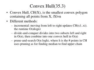
Convex Hull (35.3). Convex Hull, CH(X), is the smallest convex polygon containing all points from X, |X|=n Different methods: incremental: moving from left to right updates CH(x1..xi). the runtime O(nlogn)

E N D
Convex Hull(35.3) • Convex Hull, CH(X), is the smallest convex polygon containing all points from X, |X|=n • Different methods: • incremental: moving from left to right updates CH(x1..xi). the runtime O(nlogn) • divide-and-conquer divides into two subsets left and right in O(n), then combine into one convex hull in O(n) • prune-and-search O(n logh), where h is the # points in CH uses pruning as for finding median to find upper chain
Graham’s Scan (35.3) O(nlogn)
Finding the Closest Pair(35.4) • Brute-force: O(n2) • Divide-and-conquer algorithm with recurrence T(n)=2T(n/2)+O(n) • Divide: divide into almost equal parts by a vertical line which divides given x-sorted array X into 2 sorted subarrays • Conquer: Recursively find the closest pair in each half of X. Let = min{left, right} • Combine: The closest pair is either in distance or a pair of points from different halves.
Combine in D-a-C (35.4) • Subarray Y’ (y-sorted) of Y with points in 2 strip • pY’ find all in Y’ which are closer than in • no more than 8 in 2 rectangle • no more than 7 points can be closer than in • If the closest in the strip closer then it is the answer 2 2 left right
Voronoi Graph • Voronoi region Vor(p) (p in set S) • the set of points on the plane that are closer to p than to any othe rpoint in S • Voronoi Graph VOR(S) • dual to voronoi region graph • two points are adjacent if their voronoi regions have common contiguous boundary (segment)
Voronoi Graph • Voronoi Graph in the rectilinear plane • Rectilinear distance: p = (x, y); p’=(x’,y’) Voronoi region of b ab b a bc c ac
NP-Completeness (36.4-5) • P: yes and no in pt • NP: yes in pt • NPH NPC NP-hard NPC P NP
x x’ a’ z z’ x y’ a y Independent Set • Independent set in a graph G: pairwise nonadjacent vertices • Max Independent Set is NPC • Is there independent set of size k? • Construct a graph G: • literal -> vertex • two vertices are adjacent iff • they are in the same clause • they are negations of each other • 3-CNF with k clauses is satisfiable iff G has independent k-set • assign 1’s to literals-vertices of independent set • Example: f = (x+z+y’) & (x’+z’+a) & (a’+x+y) x, z’, y independent F is satisfiable: f = 1 if x = z’ = y = 1
red independent set MAX Clique • Max Clique (MC): • Find the maximum number of pairwise adjacent vertices • MC is in NP • for the answer yes there is certificate of polynomial length = clique which can be checked in polynomial time • MC is in NPC • Polynomial time reduction from MIS: • For any graph G any independent set in G 1-1 corresponds to clique in the complement graph G’ red clique noedge edge edge noedge G Complement G’
Minimum Vertex Cover • Vertex Cover: • the set of vertices which has at least one endpoint in each edge • Minimum Vertex Cover (MVC): • the set of vertices which has at least one endpoint in each edge • MIN Vertex Cover is NPC • If C is vertex cover, then V - C is an independent set red independent set blue vertex cover
Set Cover • Given: a set X and a family F of subsets of X, F 2X, s.t. X covered by F • Find : subfamily G of F such that G covers X and |G| is minimize • Set Cover is NPC • reduction from Vertex Covert • Graph representation: edge between set A F and element x X means x A d a b c red elements of ground set X blue subsets in family F A B A = {a,b,c}, B = {c,d}
NP-hard NPC P NP Intermediate Classes Dense Set Cover is NP but not in P neither in NPC Dense Set Cover: Each element of X belongs to at least half of all sets in F
Runtime Complexity Classes • Example • adding an element in a queue/stack • inverse Ackerman function = O(loglog…log n) n times • extracting minimum from binary heap • n1/2 • traversing binary search tree, list • O(n log n) sorting n numbers, closest pair, MST, Dijkstra shortest paths • adding two nn matrices • en ^ (1/2) • en, , n! • Ackerman function • Runtime order: • constant • almost constant • logarithmic • sublinear • linear • pseudolinear • quadratic • polynomial • subexponential • exponential • superexponential 2 . . . 2 2 n times
Hamiltonian Cycle and TSP • Hamiltonian Cycle: • given an undirected graph G • find a tour which visits each point exactly once • Traveling Salesperson Problem • given a positive weighted undirected graph G (with triangle inequality = can make shortcuts) • find a shortest tour which visits all the vertices • HC and TSP are NPC • NPC problems: SP, ISP, MCP, VCP, SCP, HC, TSP
Approximation Algorithms (37.0) • When problem is in NPC try to find approximate solution in polynomial-time • Performance Bound = Approximation Ratio (APR) (worst-case performance) • Let I be an instance of a minimization problem • Let OPT(I) be cost of the minimum solution for instance I • Let ALG(I) be cost of solution for instance I given by approximate algorithm ALG APR(ALG) = max I {ALG(I) / OPT(I)} • APR for maximization problem = max I {ALG(I) / OPT(I)}
Vertex Cover Problem (37.1) • Find the least number of vertices covering all edges • Greedy Algorithm: • while there are edges • add the vertex of maximum degree • delete all covered edges • 2-VC Algorithm: • while there are edges • add the both ends of an edge • delete all covered edges • APR of 2-VC is at most 2 • e1, e2, ..., ek - edges chosen by 2-VC • the optimal vertex cover has 1 endpoint of ei • 2-VC outputs 2k vertices while optimum k
2-approximation TSP (37.2) • Given a graph G with positive weights Find a shortest tour which visits all vertices • Triangle inequality w(a,b) + w(b,c) w(a,c) • 2-MST algorithm: • Find the minimum spanning tree MST(G) • Take MST(G) twice: T = 2 MST(G) • The graph T is Eulerian - we can traverse it visiting each edge exactly once • Make shortcuts • APR of 2-MST is at most 2 • MST weight weight of optimum tour • any tour is a spanning tree, MST is the minimum
3/2-approximation TSP (Manber) • Matching Problem (in P) • given weighted complete (all edges) graph with even # vertecies • find a matching (pairwise disjoint edges) of minimum weight • Christofides’s Algorithm (ChA) • find MST(G) • for odd degree vertices find minimum matching M • output shortcutted T = MST(G) + M • APR of ChA is at most 3/2 • |MST| OPT • |M| OPT/2 • |T| (3/2) OPT odd
3/2-approximation TSP • Christofides’s Algorithm (ChA) • find MST(G) • for odd degree vertices find minimum matching M • output shortcutted T = MST(G) + M • The worst case for Christofides heuristic in Euclidean plane: - Minimum Spanning Tree length = 2k - 2 - Minimum Matching of 2 odd degree nodes = k - 1 - Christofides heuristic length = 3k - 3 - Optimal tour length = 2k - 1 - Approximation Ratio of Christofides = 3/2-1/(k-1/2) 1 k+1 k+2 k+3 … 2k-1 1 1 2 3 4 … k 1
Non-approximable TSP (37.2) • Approximating TSP w/o triangle inequality is NPC • any c-approximation algorithm can solve Hamiltonian Cycle Problem in polynomial time • Take an instance of HCP = graph G • Assign weight 0 to any edge of G • Complete G up to complete graph G’ • Assign weight 1 to each new edge • c-approximate tour can use only 0-edges - so it gives Hamiltonian cycle of G
Euclidean metric Steiner Point Cost = 2 1 1 Cost = 3 Terminals 1 1 1 Rectilinear metric Cost = 6 Cost = 4 1 1 1 1 1 1 1 1 1 1 Steiner Tree Problem Given: A set S of points in the plane = terminals Find:Minimum-cost tree spanning S = minimum Steiner tree
Steiner Tree Problem in Graphs • Given a graph G=(V,E,cost) and terminals S in V Find minimum-cost tree spanning all terminals • MST algorithm (does not use Steiner points): • find G(S) = complete graph on terminals • edge cost = shortest path cost • find T(S) = MST of G(S) • replace each edge of T(S) with the path in G • output T(S)
MST -Heuristic Theorem: MST-heuristic is a 2-approximation in graphs Proof: MST<Shortcut TourTour = 2 • OPTIMUM
Approximation Ratios • Euclidean Steiner Tree Problem • approximation ratio = 2/3 • Rectilinear Steiner Tree Problem • approximation ratio = 3/2 • Steiner Tree Problem in graphs • approximation ratio = 2 1 MST Cost = 2k-2 2 3 Opt Cost = k Steiner Point Approximation ratio = 2-2/k 2 4 k 5
The Set Cover Problem • Sets Aicover a set X if X is a union of Ai • Weighted Set Cover Problem Given: • A finite set X (the ground set X) • A family of F of subsets of X, with weights w: F + Find: • sets S F, such that • S covers X, X = {s | s S} and • S has the minimum total weight {w(s) | s S} • If w(s) =1 (unweighted), then minimum # of sets
Greedy Algorithm for SCP 1 • Greedy Algorithm: • While X is not empty • find s F minimizing w(s) / |s X| • X = X - s • C = C + s • Return C 2 6 3 4 5
Analysis of Greedy Algorithm • Th: APR of the Greedy Algorithm is at most 1+ln k • Proof:
Approximation Complexity • Approximation algorithm = polynomial time approximation algorithm • PTAS = a series of approximation algorithms s.t. for any > 0 there is pt (1+)-approximation • There is PTAS fro subset sum • Remarkable progress in 90’s (assuming P NP). • No PTAS for Vertex Cover • No clog k-approximation for Set Cover for k < 1 • k is the size of the ground set X • No n1- approximation for Independent Set • n is the number of vertices