Download
1 / 23
230 likes | 376 Views
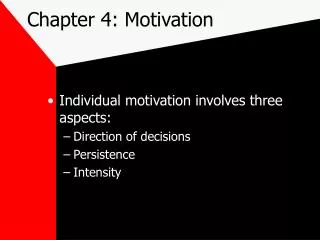
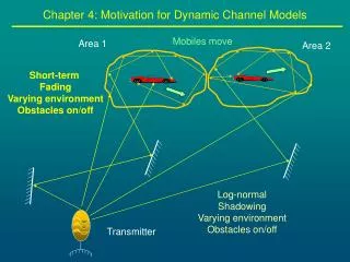
Chapter 4: Motivation for Dynamic Channel Models. Mobiles move. Area 1. Area 2. Short-term Fading Varying environment Obstacles on/off. Log-normal Shadowing Varying environment Obstacles on/off. Transmitter. Chapter 4: Motivation for Dynamic Channel Models.

E N D
Chapter 4: Motivation for Dynamic Channel Models Mobiles move Area 1 Area 2 Short-term Fading Varying environment Obstacles on/off Log-normal Shadowing Varying environment Obstacles on/off Transmitter
Chapter 4: Motivation for Dynamic Channel Models • Complex low-pass representation of impulse response:
Chapter 3: S.D.E.’s for Short-Term Fading • Dynamics represent time-variations of environment • Captured by Doppler power spectrum • From power spectral densities to S.D.E.’s • State-space realizations of In-phase and Quadrature components • Time-domain simulations flat-fading, frequency select. • Distributions of short-term dynamical channel • Summary of distributions
Chapter 3: 3-Dimensional Scattering Model z z0 nth incoming wave En=:{rn,fn,an,bn}; n=1,…, N O’(x0 ,y0 ,z0) bn O an x x0 y0 g O’’ v y direction of motion of mobile on x-y plane • 3-Dimensional Model[Clarke 68, Aulin 79]
Chapter 3: Doppler P.S.D. is Band-limited • Doppler Power Spectral Density • Factorization (Normalization, Approximation) • State-Space Model • Doppler Power Spectral Density • Factorization (Normalization, Approximation) • State-Space Model
Chapter 4: Power Spectral Densities and S.D.E.’s Gaussian process Gaussian process LTI Ryy(Dt) Rxx(Dt) WSS x(t) y(t) Sxx(w) |H(w)|2 Syy(w) x = • Power Spectral Density: Syy(w)=Ft[Ryy(Dt)] Linear system h(t)
Chapter 4: Factorization of Approximated P.S.D. • Factorization
Chapter 4: Approximate P.S.D. • Approximation
Chapter 4: State-space realizations of Fading Process • Nominal state-space model
Chapter 4: State-Space Realizations of Fading Process • Nominal state-space model: mean and variance
Chapter 4: T.-D. Simulations of Fading Process cos wct sin wct ABCD ABCD delay dWQ dWI s(t) + y(t) + - Flat-Fading Channel X X X • Nominal state-space model
Chapter 4: T.-D. Simulations of Fading Process Experimental Data (Pahlavan) • Simulation of Flat-Fading Channel using Matlab
Chapter 4: T.-D. Simulations of Fading Process • Simulation of frequency-selective Channel using Matlab
Chapter 4: T.-D. Simulations of Fading Process • Simulation of received signal through a frequency-selective channel using Matlab
Chapter 4: T.-D. Simulations of Fading Process • Temporal simulations of received signal for a multipath channel: • From PSD obtain parameters of state-space model. • Dynamics of channel gain obtained through solving state-space model (generate independent brownian motions for in-phase and quadrature components). • Identify the parameters of the non-homogeneous Poisson process l(t). This characterizes the obstacles in the environment. • Generate points of non-homogeneous poisson process. This corresponds to generating the path arrival times. • Associate each path with a gain computed using the state-space model.
Chapter 4: Shot-Noise Model Simulations • Temporal simulations of received signal:
Chapter 4: Probability Distributions of Attenuations • Probability Distribution – Rayleigh: an(t)=0.
Chapter 4: Probability Distributions of Attenuations Non-Stationary Rician Non-Stationary Nakagami n=2 n=2 Xj(s)= 0,gj = 0 j =1,…,n X1(s)= X2 (s)= 0 g1= g2 =0 a=0 n=2 Stationary Rician Stationary Nakagami Non-Stationary Rayleigh t large Stationary Rayleigh a and/or t large n=2 g1= g2 =0
Signature Functions & Parameters 50 1 25 Correlation Relative Power 0 0 -1 -80 - 60 -40 -20 0 20 40 60 80 -0.1 0 0.1 Frequency (Hz) Lag (S) Autocorrelation Power Spectral Density Re: Paper of R. Bultitude et al. from URSI G.A. CRC-TU/e-TU/d-U/Ottawa
Chapter 4: References • E. Wong, B. Hajek. Stochastic Processes in Engineering Systems. Springer-Verlag, New York, 1985. • M.C. Jeruchim, P. Balaban, S. Shanmugan. Simulation of Communication Systems. Plenum, New York, 1994. • P. E. Kloeden, E. Platen. Numerical Solution of Stochastic Differential Equations. Springer-Verlag, New York, 1999. • C.D. Charalambous, N. Menemenlis. Stochastic models for short-term multipath fading: Chi-Square and Ornstein-Uhlenbeck processes. Proceedings of 38th IEEE Conference on Decision and Control, 5:4959-4964, December 1999. • C.D. Charalambous, N. Menemenlis. Multipath channel models for short-term fading. 1999 International Workshop on mobile communications, pp 163-172, Creta, Greece, June 1999. • C.D. Charalambous, N. Menemenlis. A state-space approach in modeling multipath fading channels via stochastic differntial equations. ICC-2001 International Conference on Communications, 7:2251-2255, June 2001.