Download
1 / 58
580 likes | 639 Views
UNIT IV: INFORMATION & WELFARE. Decision under Uncertainty Bargaining Externalities & Public Goods Review. 11 / 9. Strategic Competition. From Last Time:. Dominance Reasoning Best Response and Nash Equilibrium Mixed Strategies Repeated Games The Folk Theorem Cartel Enforcement.

E N D
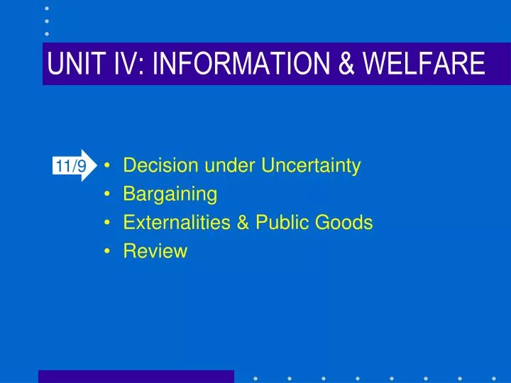
UNIT IV: INFORMATION & WELFARE • Decision under Uncertainty • Bargaining • Externalities & Public Goods • Review 11/9
Strategic Competition From Last Time: • Dominance Reasoning • Best Response and Nash Equilibrium • Mixed Strategies • Repeated Games • The Folk Theorem • Cartel Enforcement
Cartel Enforcement Consider a market in which two identical firms can produce a good with a marginal cost of $1 per unit. The market demand function is given by: P = 7 – Q Assume that the firms choose prices. If the two firms choose different prices, the one with the lower price gets all the customers; if they choose the same price, they split the market demand. What is the Nash Equilibrium of this game?
Cartel Enforcement Demand Condition: P = 7 – Q; Supply Condition: TCi= qi MR = MC Monopoly TR = PQ = (7-Q)Q = 7Q - Q2 MR = 7-2Q = MC =1 • Qm= 3; Pm = 4 $ Pm=4 MC D MR Q Qm=3
Cartel Enforcement Demand Condition: P = 7 – Q; Supply Condition: TCi= qi MR = MCQ = q1 + q2 Monopoly Cournot Duopoly Bertrand Duopoly TR = PQ = (7-Q)Q tr1 = P(q1) = 7q1 - q12 - q1q2 = 7Q - Q2 mr = 7 - 2q1 - q2 = mc1 = 1 MR = 7-2Q = MC =1 q1* = 3 - ½ q2 q2* = 3 - ½ q1 = 3 - ½(3 - ½ q2) => q2* = 2 = q1* Qm = 3; Pm = 4Qc= 4; Pm = 3 Qb = 6; Pb = 1
Cartel Enforcement Consider a market in which two identical firms can produce a good with a marginal cost of $1 per unit. The market demand function is given by: P = 7 – Q Now suppose that the firms compete repeatedly, and each firm attempts to maximize the discounted value of its profits ( < 1). What if this pair of Bertrand duopolists try to behave as a monopolist (w/2 plants)?
Cartel Enforcement What if a pair of Bertrand duopolists try to behave as a monopolist (w/2 plants)? P = 7 – Q; TCi = qi MonopolyBertrand Duopoly • = TR – TC Q = q1 + q2 = PQ – Q Pb = MC = 1; Qb = 6 = (7-Q)Q - Q = 7Q - Q2 - Q FOC: 7-2Q-1 = 0 => Qm = 3; Pm = 4 w/2 plants: q1 = q2 = 1.5 q1 = q2 = 3 P1= P2 = 4.5 P1= P2 = 0
Cartel Enforcement What if a pair of Bertrand duopolists try to behave as a monopolist (w/2 plants)? Promise: I’ll charge Pm = 4, if you do. Threat: I’ll charge Pb = 1, forever, if you deviate. 4.5 … 4.5 … 4.5 … 4.5 … 4.5 … 4.5 … 4.5 = 4.5/(1-d) 4.5 … 4.5 … 4.5 … 9 … 0 … 0 … 0 If d is sufficiently high, the threat will be credible, and the pair of trigger strategies is a Nash equilibrium. Trigger Strategy Current gain from deviation = 4.5
Cartel Enforcement What if a pair of Bertrand duopolists try to behave as a monopolist (w/2 plants)? I’ll charge Pm if you do. I’llcharge mc, forever, if you deviate. 4.5 … 4.5 … 4.5 … 4.5 … 4.5 … 4.5 … 4.5 = 4.5/(1-d) 4.5 … 4.5 … 4.5 … 9 … 0 … 0 … 0 If d is sufficiently high, the threat will be credible, and the pair of trigger strategies is a Nash equilibrium. d* = 0.5 Trigger Strategy Current gain from deviation = 4.5 Future gain from cooperation = d(4.5)/(1-d)
Cartel Enforcement What if a pair of Bertrand duopolists try to behave as a monopolist (w/2 plants)? Promise: I’ll charge Pm = 4, if you do. Threat: I’ll charge Pb = 1, forever, if you deviate. R … R … R … R … R … R … R= R/(1-d) R … R … R … T … P … P… P If d is sufficiently high, the threat will be credible, and the pair of trigger strategies is a Nash equilibrium. d* = (T-R)/(T-P) Trigger Strategy Current gain from deviation = T-R Future gain from cooperation = d(R-P)/(1-d)
The Folk Theorem Theorem: Any payoff that pareto-dominates the one-shot NE can be supported in a SPNE of the repeated game, if the discount parameter is sufficiently high. (S,T) (R,R) (P,P) (T,S)
The Folk Theorem In other words, in the repeated game, if the future matters “enough” i.e., (d > d*), there are zillions of equilibria! (S,T) (R,R) (P,P) (T,S)
The Folk Theorem • The theorem tells us that in general, repeated games give rise to a very large set of Nash equilibria. In the repeated PD, these are pareto-rankable, i.e., some are efficient and some are not. • In this context,evolution can be seen as a process that selects for repeated game strategies with efficient payoffs. “Survival of the Fittest”
UNIT IV: INFORMATION & WELFARE • Decision under Uncertainty • Externalities & Public Goods • Review
Decision under Uncertainty In UNIT I we assumed that consumers have perfect information about the possible options they face (their income and prices); and about the utility consequences of their choices (their preferences). Now, we will ask whether our model can be extended to deal with more realistic cases in which decisions are made without perfect information. We will also ask how imperfect (asymmetric) information affects market outcomes and their welfare consequences.
Decision under Uncertainty The Economics of Information: How can I maximize utility given incomplete info? How much info should I gather? We can distinguish between 2 sources of uncertainty: • The behavior of other actors (strategic uncertainty) • states of nature (natural uncertainty) • Will it rain? Or not? • Is there oil in the drilling hole? • Will the roulette wheel come up red? (1 -- 35) • Is the car a lemon?
Decision under Uncertainty The Economics of Information: How can I maximize utility given incomplete info? How much info should I gather? We can distinguish between 2 sources of uncertainty: • states of nature (natural uncertainty) • Will it rain? Or not? • Is there oil in the drilling hole? • Will the roulette wheel come up red? (1 -- 35) • Is the car a lemon?
Decision under Uncertainty • Expected Value v. Expected Utility • Risk Preferences • Reducing Risk: Insurance • Contingent Consumption • Adverse Selection (and Moral Hazard)
Expected Value & Expected Utility Which would you prefer? A) 50-50 chance of winning $30,000 or losing $5,000 B) Sure thing of $10,000
Expected Value & Expected Utility How much would you be willing to pay for the chance to win $2n if a heads comes up on nth flip? Expected Value (EV): the sum of the value (V) of each possible state, weighted by the probability (p) of that state occurring. On 1 flip: p(H) = ½
Expected Value & Expected Utility How much would you be willing to pay for the chance to win $2n if a heads comes up on nth flip? Expected Value (EV): the sum of the value (V) of each possible state, weighted by the probability (p) of that state occurring. On 1 flip: EV = p(V)H = (½)2
Expected Value & Expected Utility How much would you be willing to pay for the chance to win $2n if a heads comes up on nth flip? Expected Value (EV): the sum of the value (V) of each possible state, weighted by the probability (p) of that state occurring. On nth flip: EV(Hn) = ½n(2n)
Expected Value & Expected Utility How much would you be willing to pay for the chance to win $2n if a heads comes up on nth flip? H T EV(H)=½(2)+(1/4)4+(1/8)8 Flip 1: Win $2 ½ ½ H T Flip 2: Win $4 ¼ ¼ H T Flip 3: Win $8 ½ 8 8
Expected Value & Expected Utility How much would you be willing to pay for the chance to win $2n if a heads comes up on nth flip? Expected Value (EV): the sum of the value (V) of each possible state, weighted by the probability (p) of that state occurring. On n flips: EV(H)=(½)2+(1/4)4+(1/8)8+…=1+1+1+…= infinity So, you’d be willing to pay an awful lot? What’s going on here?
Expected Value & Expected Utility With examples such as these, David Bernoulli (1738) observed that rational agents often behave contrary to expected value maximization. Instead, they maximize: Expected Utility (EU): the sum of the utility of each possible state, weighted by the probability of that state occurring. EU = p1(U(s1)) + p2(U(s2)) + … pn(U(sn)) Where p is the probability of that state occurring.
Expected Value & Expected Utility With examples such as these, David Bernoulli (1738) observed that rational agents often behave contrary to expected value maximization. Instead, they maximize: Expected Utility (EU): the sum of the utility of each possible state, weighted by the probability of that state occurring. Rankings of expected values and expected utilities need not be the same! Differences arise because utility will be a non-linear function of “wealth” and will depend on endowments. * * or “income” or “consumption”
Expected Value & Expected Utility Diminishing Marginal Utility: The intrinsic worth of wealth increases with wealth, but at a diminishing rate. U U(15) U(10) U(5) von Neumann-Morgenstern Utility Indexes MU = ½W-½ U = W½ MU = 1/W U = lnW For 2 states: EU = p(U(Wi)) + (1-p)(U(Wj)) MRS = (p/(1-p))MUi/MUj 5 10 15 W
Risk Preferences A risk averse consumer will prefer a certain income to a risky income with the same expected value. U U(15) U(10) U(5) The chord represents the chance to win $5 or $15. .5U(5) +.5U(15) 5 CE 10 15 W
Risk Preferences A risk averse consumer will prefer a certain income to a risky income with the same expected value. U U(15) U(10) U(5) Certainty Equivalent (CE) of an equal chance of winning $5 and $15 Risk Premium = 10 – CE .5U(5) +.5U(15) 5 CE 10 15 W
Risk Preferences A risk loving consumer will prefer a risky income to a certain income with the same expected value. U U(15) .5U(5) +.5U(15) U(5) U(10) 5 CE 10 15 W
Risk Preferences A risk neutral consumer is indifferent between a risky income and a certain income with the same expected value. U U(15) U(10) U(5) 5 CE 10 15 W
Risk Preferences A risk neutral consumer is indifferent between a risky income and a certain income with the same expected value. Do any of these cases violate any of our assumptions about well-behaved preferences? Draw a set of indifference curves for each case. U U(15) U(10) U(5) 5 CE 10 15 W
Risk and Insurance A risk averse consumer will prefer a certain income to a risky income with the same expected value. Given the opportunity, therefore, she will attempt to smooth the variability of her wealth, by spreading (or diversifying) her risks across states. Insurance offers a way to buy wealth in the event of a low wealth (or “bad”) state, by transferring some wealthfrom the “good” to the “bad” state.
Risk and Insurance A risk averse consumer has wealth of $35,000, including a car worth $10,000. There is a 1/100 chance that the car will be stolen. So there is a 0.01 chance his wealth will be $25,000 and a 0.99 chance it will be $35,000. EW = 0.01(25000) + 0.99(35000) Buying insurance can change this distribution.
Risk and Insurance If his car is stolen, his wealth will be $25,000; if it is not stolen, his wealth will be $35,000. Buying insurance is transferring wealth from the “good” to the “bad” state. Wg $35,000 Suppose he can by $1000 insurance at a premium of $1/100. g = .01 How much insurance will he buy? ? $25,000 Wb
Risk and Insurance If his car is stolen, his wealth will be $25,000; if it is not stolen, his wealth will be $35,000. Buying insurance is transferring wealth from the “good” to the “bad” state. Wg $35,000 Given the chance to buy insurance at an “actuarily fair” price (i.e., g = p), a risk averse consumer will fully insure. Equalizing wealth across states. Certainty Line 34,900 $25,000 Wb 34,900
Risk and Insurance Insurance is a way to allocate wealth across possible states of the world. In essence, he is purchasing contingent claims on consumption (wealth) in the two states. So we can solve in the usual way: Wg Eg Endowment More generally: E =Endowment K = dollars of insurance g = premium ? Eg - gK Eb Wb Eb + K - gK
Contingent Consumption If his car is stolen, his wealth will be $25,000; if it is not stolen, his wealth will be $35,000. Buying insurance is transferring wealth from the “good” to the “bad” state. Wg $35,000 Endowment Now suppose the premium rises to $1.10/100 (g = .011). His vN-M Index: U = lnW How much insurance will he buy? 35000 - gk $25,000 Wb 25,000 + K - gK
Contingent Consumption If his car is stolen, his wealth will be $25,000; if it is not stolen, his wealth will be $35,000. Buying insurance is transferring wealth from the “good” to the “bad” state. Wg $35,000 Slope(m) = DWg/DWb = -gK/(K-gK) = -g/(1-g) g = Pb 1-g = Pg m = -Pb/Pg $25,000 Wb Not to scale
Contingent Consumption If his car is stolen, his wealth will be $25,000; if it is not stolen, his wealth will be $35,000. Buying insurance is transferring wealth from the “good” to the “bad” state. Wg $35,000 What is his budget constraint? Wg* m = -.0111 $25,000 Wb Wb* Not to scale
Contingent Consumption If his car is stolen, his wealth will be $25,000; if it is not stolen, his wealth will be $35,000. Buying insurance is transferring wealth from the “good” to the “bad” state. Wg $35,000 Budget Constraint: Wg = m(Wb) + Wg(int) Wg = -(.011/.989)Wb + 35278 Wg* m = -.0111 $25,000 Wb Wb* Not to scale
Contingent Consumption If his can is stolen, his wealth will be $25,000; if it is not stolen, his wealth will be $35,000. Buying insurance is transferring wealth from the “good” to the “bad” state. Wg $35,000 MRS = (.01/.99)(Wg/Wb) Pb/Pg = g/(1-g) MRS = Pb/Pg => Wb = .909Wg Wg = -(.011/.989)Wb + 35278 Wg = $ 34925 Wg* $25,000 Wb Wb* Not to scale
Contingent Consumption If his can is stolen, his wealth will be $25,000; if it is not stolen, his wealth will be $35,000. Buying insurance is transferring wealth from the “good” to the “bad” state. Wg $35,000 Wg = $ 34925 So he pays $75 for $6818 of ins Wg*=34925 $25,000 Wb Wb*=31743 Not to scale
Contingent Consumption How would the answer change for a risk lover? Wg Eg A risk lover will maximize utility (reach her highest indifference curve) in a corner solution. In this case, remaining at the endowment. Eb Wb
Adverse Selection Consider the market for drivers insurance: “Good” drivers have accidents with prob = 0.2 “Bad”= 0.8 Good and bad drivers are equally distributed in population. ” What price would an actuarially fair insurance company charge?
Adverse Selection Consider the market for drivers insurance: “Good” drivers have accidents with prob = 0.2 “Bad” = 0.8 Good and bad drivers are equally distributed in population. At the actuarially fair price of $0.50/$1 coverage: • for good drivers price is too high -> don’t insure • for bad too low -> insure Bad drivers are “selected in”; good are “selected out” Driver quality is a hidden characteristic
Adverse Selection Consider the market for drivers insurance: “Good” drivers have accidents with prob = 0.2 “Bad” = 0.8 Good and bad drivers are equally distributed in population. At the actuarially fair price of $0.50/$1 coverage: • for good drivers price is too high -> don’t insure • for bad too low -> insure Bad drivers are “selected in”; good are “selected out” Asymmetric Information
Acquiring a Company BUYER represents Company A (the Acquirer), which is currently considering make a tender offer to acquire Company T (the Target) from SELLER. BUYER and SELLER are going to be meeting to negotiate a price. Company T is privately held, so its true value is known only to SELLER. Whatever the value, Company T is worth 50% more in the hands of the acquiring company, due to improved management and corporate synergies. BUYER only knows that its value is somewhere between 0 and 100 ($/share), with all values equally likely. Source: M. Bazerman
Acquiring a Company What offer should Buyer make?
Acquiring a Company 45 123 BU MBA Students Similar results from MIT Master’s Candidates CPA; CEOs. Source: Bazerman, 1992 27 18 9 7 4 5 4 1 0 $0 10-15 20-25 30-35 40-45 50-55 60-65 70-75 80-85 90-95 Offers