Download

1 / 17
180 likes | 362 Views
Notes 7: Function Optimization. ICS 171 Winter 2000. Example 1: The “Travelling Salesman Problem”. Problem Statement: there are N cities and N 2 costs of travelling between any 2 cities A tour from city A, is a path starting at city A, visiting all cities once, and ending back at city A

E N D
Notes 7: Function Optimization ICS 171 Winter 2000
Example 1: The “Travelling Salesman Problem” • Problem Statement: • there are N cities and N2 costs of travelling between any 2 cities • A tour from city A, is a path starting at city A, visiting all cities once, and ending back at city A • note: this is not a state-space! “states” = possible tours (N! of them) • Find the shortest tour from A A
Example 2: Intel chip manufacturing • Consider the following hypothetical problem • x = sales price of Intel’s newest chip (in $1000’s of dollars) • F(x) = profit per chip (in $1000’s of dollars). • Assume that Intel’s marketing research team has found that the profit per chip (as a function of x) isF(x) = x2 - x3 • Assume that we must have x non-negative and no greater than 1 • Set this up as an optimization problem: • objective function is profit F(x) that needs to be maximized • solution to the optimization problem will be the optimum chip sales price
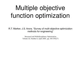
Example 3: Regression Y Find the best line Y=aX+b describing the set of given points (xi,yi) X The problem boils down to finding distances from individual points to the line and minimizing the sum of these distances as a function of parameters a nd b defining the line.
General Statement of Optimization Problem or where x - input variable, scalar or vector valued D - domain for x over which optimization is performed F - objective function, can be computed or known analytically Note: we can always replace maximization problem with an equivalent minimization problem, so in what follows we discuss only minimization problems
Important Notes for Optimization Problems • We are interested in knowing those points x0 from D in the neighborhood of which F(x) > F(x0), I.e. x0 is a minimum. Compare this to search --- we the path to the goal was solution. • We will discuss local Vs global minimum. The latter is the lowest value of F for all x in D and is usually much harder to find. • Optimization is a very difficult problem in general, especially when x is high dimensional, unless F is simple (e.g. linear) and known analytically. • The methods of finding a minimum of F can be divided into analytical (work when F is known analytically) and numerical (work for any F). We consider a few popular methods in what follows.
Analytical Method: Differentiating Assume F is known analytically and twice differentiable.The critical points of F, ie the points of potential maximum or minimum, are given by equation (1) Once the roots x1, x2, …., xN of (1) are found, the sign of the second derivative tells if each of those points is a maximum or a minimum: for x=xj, then x=xj is a minumum If for x=xj, then x=xj is a maximum If If the second derivative is 0 in a critical point xj then xj may or may not be a minimum or a maximum of F. WHY?
0.15 f(x) 0.0 1.0 0.0 x Differentiating: Solving Intel Manuf. Example • Since we know f(x) analytically, we can find d/dx f(x) = 2x - 3x2 • Setting this to 0, we get 2x = 3x2 and hencex0 = 2/3 is a critical point • d2/dx2 f(x) =2-6x, and, when x=x0=2/3, we have d2/dx2 f(x0) = -2 < 0, so x0 is a maximum • So, the optimal price per chip is $667 maximizes the profit
Properties of Differentiating • Generalizes to a high dimensional case --- will need to take partial derivatives in each dimension and solve a system of equations of type (1). • For a bounded D the only possible points of maximum/minimum are critical or boundary ones, so, in principle, we can find the global extremum. • Potential problems include transcendent equation (1), not solvable analytically, high cost of finding derivatives, especially in high dimensions (e.g. for neural networks) • Partial Solution of the problems comes from a numerical technique called the gradient descent discussed on the next few slides
Numerical Method: Gradient Descent For analytical and smooth objective function F and the currently picked x0 from D, we want to chose x in the neighborhood of x0 so that F(x) < F(x0). Applying Taylor’s expansion in the neighborhood of x0 we get If we discard the terms of the second and higher orders, and enforce F(x) < F(x0) we will get: The last inequality is easy to satisfy by setting - gradient descent method
Properties of Gradient Descent f(x) x Iterative method, starts from a random point, and from the point obtained on the previous iteration makes a small move in the direction of the most rapid function decrease - antigradient. Generalizes straightforwardly to high dimensions, partial derivatives are taken for each of the independent variables Gradient Descent is one of the most practical methods if the derivative or its numerical estimate is available (usually the case) Guaranteed to find a local minimum with a sufficiently small step , random restarts are usually used to improve the solution
Numerical Method: Minima Localization using Grid • Evaluate objective function in xj=A+j*B, where D=[A,B]. Then chose min F(xj) and declare it the starting point for the gradient descent search • Main problem: suppose x is 10 dimensional, want at least 10 points in each dimension ---> how many points to evaluate F at? 1010 -- enormous!
Solving the Travelling Salesman Problem • This is a classic problem • models many practical problems • e.g., minimum number of movements for industrial machines • scales exponentially in N • however various heuristic search algorithms work well in practice • e.g., descent (greedy): start with a random tour and change the link which gives the greatest decrease in tour cost. • however, descent can have local minima/maxima • Optimality and Near-optimal solutions • for many problems finding the single best solution is NP-hard • However, in practice, from an engineering viewpoint, we may be satisfied with quickly finding “nearly optimal” solutions. • so descent to local maxima may be ok in practice
Numerical Method: Simulated Annealing • Simulated Annealing = descent with non-deterministic search • Basic ideas: • like descent identifies the quality of the local improvements • instead of picking the best move, pick one randomly • say the change in objective function is d • if d is negative, then move to that state • otherwise: • move to this state with probability proportional to d • thus: worse moves (very large positive d) are executed less often • however, there is always a chance of escaping from local minima • over time, make it less likely to accept locally bad moves • (Can also make the size of the move random as well, i.e., allow “large” steps in state space)
Physical Interpretation of Simulated Annealing • A Physical Analogy: • imagine letting a ball roll downhill on the function surface • this is like descent (for minimization) • now imagine shaking the surface, while the ball rolls, gradually reducing the amount of shaking • this is like simulated annealing • Annealing = physical process of cooling a liquid or metal until particles achieve a certain frozen crystal state • simulated annealing: • free variables are like particles • seek “low energy” (high quality) configuration • get this by slowly reducing temperature T, which particles move around randomly
More Details on Simulated Annealing • Lets say there are 3 moves available, with changes in the objective function of d1 = 0.1, d2 = -0.5, d3 = 5. (Let T = 1). • pick a move randomly: • if d2 is picked, move there. • if d1 or d3 are picked, probability of move = exp(-d/T) • move 1: prob1 = exp(-0.1) = 0.9, • i.e., 90% of the time we will accept this move • move 3: prob3 = exp(-5) = 0.05 • i.e., 5% of the time we will accept this move • T = “temperature” parameter • high T => probability of “locally bad” move is higher • low T => probability of “locally bad” move is lower • T = 0 => we get hill-climbing • typically, T is decreased as the algorithm runs longer • i.e., there is a “temperature schedule”
Properties of Simulated Annealing • With an optimal temperature schedule guaranteed to find global minimum of the objective function --- great! Although how do we find the optimal schedule? In practice we just know that slower temperature decreases, the higher quality solution we will get. • Very cheap to implement, often a method of choice in high dimensions. • Converges slowly because of the slow decrease in temperature, but can always report “the-best-so-far” solution.