Download
1 / 61
630 likes | 775 Views
CLUSTERING ALGORITHMS VIA FUNCTION OPTIMIZATION. In this context the clusters are assumed to be described by a parametric specific model whose parameters are unknown (all parameters are included in a vector denoted by θ ) . Examples:

E N D
CLUSTERING ALGORITHMS VIA FUNCTION OPTIMIZATION • In this context the clusters are assumed to be described by a parametric specific model whose parameters are unknown (all parameters are included in a vector denoted by θ). Examples: • Compact clusters. Each cluster Ci is represented by a point mi in the l-dimensional space. Thus θ=[m1T, m2T, …, mmT]T. • Ring-shaped clusters. Each cluster Ci is modeled by a hypersphere C(ci,ri), where ci and ri are its center and its radius, respectively. Thus θ=[c1T, r1, c2T, r2, …, cmT, rm]T. • A cost J(θ) is defined as a function of the data vectors in X and θ.Optimization of J(θ) with respect to θ results inθ that characterizes optimally the clusters underlying X. • The number of clusters m is a priori known in most of the cases.
Cost optimization clustering algorithms considered in the sequel • Mixture decomposition schemes. • Fuzzy clustering algorithms. • Possibilistic clustering algorithms.
Mixture Decomposition (MD) schemes • Here, each vector belongs to a single cluster with a certain probability • MD schemes rely on the Bayesian framework: A vector xi is appointed to cluster Cj if P(Cj| xi)>P(Ck| xi), k=1,…,m, k≠j. However: • No cluster labeling information is available for the data vectors • The a priori cluster probabilities P(Cj)Pjare also unknown • A solution: Adoption of the EM algorithm • E-step where θ=[θ1Τ,…,θmT]T (θj the parameter vector corresponding to Cj) P=[P1,…Pm]T (Pj the a priori probability for Cj) Θ=[θT, PT]T
M-step Θ(t+1)=argmaxΘQ(Θ;Θ(t)) More specifically, the M-step results in: For θj’s: (*) Provided that all pairs of (θk,θj) are functionally independent. For Pj’s: (**) Taking into account the constraints Pk0, k=1,…,m and P1+P2+…Pm=1. Thus, the EM algorithm for this case may be stated as follows:
Generalized Mixture Decomposition Algorithmic Scheme (GMDAS) • Choose initial estimates, θ=θ(0) and P=P(0). • t=0 • Repeat • Compute , i=1,…,N, j=1,…,m (1) • Set θj(t+1) equal to the solution of the equation (2) with respect to θj, for j=1,…,m. • Set ,j=1,…,m (3) • t=t+1 • Until convergence, with respect to Θ, is achieved.
Remarks: • A termination condition for GMDAS is ||Θ(t+1)-Θ(t)||<ε where ||.|| is an appropriate vector norm and ε a small user-defined constant. • The above scheme is guaranteed to converge to a global or a local maximum of the loglikelihood function. • Once the algorithm has converged, xí’s are assigned to clusters according to the Bayes rule.
Compact and Hyperellipsoidal Clusters In this case : • each cluster Cj is modeled by a normal distribution N(μj,Σj). • θj consists of the parameters of μj and the (independent) parameters of Σj. It is ,j=1,…,m For this case: • Eq. (1) in GMDAS is replaced by • Eq. (2) in GMDAS is replaced by the equations
Remark: • The above scheme is computationally very demanding since it requires the inversion of the m covariance matrices at each iteration step. Two ways to deal with this problem are: • The use of a single covariance matrix for all clusters. • The use of different diagonal covariance matrices. • Example 1: (a) Consider three two-dimensional normal distributions with mean values: μ1=[1, 1]T, μ2=[3.5, 3.5]T, μ3=[6, 1]T and covariance matrices respectively. A group of 100 vectors stem from each distribution. These form the data set X.
Results of GMDAS The data set Confusion matrix: The algorithm reveals accurately the underlying structure.
(b) The same as (a) but now μ1=[1, 1]T, μ2=[2, 2]T, μ3=[3, 1]T (The clusters are closer). The data set Results of GMDAS Confusion matrix: The algorithm reveals the underlying structure less accurately.
Fuzzy clustering algorithms • Each vector belongs simultaneously to more than one clusters. • A fuzzy m-clustering of X, is defined by a set of functions uj: X A[0, 1], j=1,…,m. If A={0,1}, a hard m-clustering of X is produced. • uj(xi) denotes the degree of membership of xi in cluster Cj. It is u1(xi)+ u2(xi)+…+ um(xi)=1 • The number of clusters m is assumed to be known a priori.
Fuzzy clustering algorithms (cont) • Cost function definition Let • θj be the representative vector of Cj. • θ[θ1T,…, θmT]T. • U[uij]=[uj(xi)] • d(xi,θj) be the dissimilarity between xi and θj • q(>1) a parameter called fuzzifier.
Fuzzy clustering algorithms (cont) • Most fuzzy clustering schemes result from the minimization of : Subject to the constraints: where uij[0,1], i=1,…,N, j=1,…,m and
Remarks: • The degree of membership of xi in Cj cluster is related to the grade of membership of xi in rest m-1 clusters. • If q=1, no fuzzy clustering is better than the best hard clustering in terms of Jq(θ,U). • If q>1, there are fuzzy clusterings with lower values of Jq(θ,U) than the best hard clustering.
Fuzzy clustering algorithms (cont) • Minimizing Jq(θ,U): Minimization Jq(θ,U) with respect to U, subject to the constraints leads to the following Lagrangian function, Minimizing JLan(θ,U) with respect to urs, we obtain Setting the gradient of J(θ,U), with respect to θ, equal to zero we obtain, The last two equations are coupled. Thus, no closed form solutions are expected. Therefore, minimization is carried out iteratively.
Generalized Fuzzy Algorithmic Scheme (GFAS) • Choose θj(0) as initial estimate for θj,j=1,…,m. • t=0 • Repeat • For i=1 to N • For j=1 to m (A) • End {For-j} • End {For-i} • t=t+1 • For j=1 to m • Parameter updating: Solve (B) with respect to θj and set θj(t) equal to this solution. • End {For-j} • Until a termination criterion is met
Remarks: • A candidate termination condition is ||θ(t)-θ(t-1)||<ε, where ||.|| is any vector norm and ε a user-defined constant. • GFAS may also be initialized from U(0) instead of θj(0), j=1,…,m and start iterations with computing θj first. • If a point xi coincides with one or more representatives, then it is shared arbitrarily among the clusters whose representatives coincide with xi, subject to the constraint that the summation of the degree of membership over all clusters sums to 1.
Fuzzy Clustering – Point Representatives • Point representatives are used in the case of compact clusters • Each θj consists of l parameters • Every dissimilarity measure d(xi,θj) between two points can be used • Common choices for d(xi,θj) are • d(xi,θj)=(xi- θj)TA(xi- θj), where A is symmetric and positive definite matrix. In this case: d(xi,θj) / θj= 2A(θj-xi). Thus the updating equation (B) in GFAS becomes • GFAS with the above distance is also known as Fuzzy c-Means (FCM) or Fuzzy k-Means algorithm. • FCM converges to a stationary point of the cost function or it has at least one subsequence that converges to a stationary point. This point may be a local (or global) minimum or a saddle point.
Fuzzy clustering – Point representatives (cont.) • The Minkowski distance where p is a positive integer and xik, θjk are the k-th coordinates of xi and θj. For even and finite p, the differentiability of d(xi,θj) is guaranteed. In this case the updating equation (B) of GFAS gives a system of l nonlinear equations with l unknowns. GFAS algorithms with the Minkowski distance are also known as pFCM algorithms.
Fuzzy Clustering – Point representatives (cont.) • Example 2(a): • Consider the setup of example 1(a). • Consider GFAS with distances (i) d(xi,θj)=(xi-θj)TA(xi-θj), with A being the identity matrix (ii) d(xi,θj)=(xi-θj)TA(xi-θj), with (iii) The Minkowski distance with p=4. • Example 2(b): • Consider the setup of example 1(b). • Consider GFAS with the distances considered in example 2(a).
The corresponding confusion matrices for example 2(a) and 2(b) are (Here a vector is assigned to the cluster for which uij has the maximum value.) For the example 2(a) For the example 2(b) • Remarks: • In Ai and Aiii (example 2(a)) almost all vectors from the same distribution are assigned to the same cluster. • The closer the clusters are, the worse the performance of all the algorithms. • The choice of matrix A in d(xi,θj)=(xi-θj)TA(xi-θj) plays an important role to the performance of the algorithm.
Fuzzy Clustering – Quadric surfaces as representatives Here the representatives are quadric surfaces (hyperellipsoids, hyperparaboloids, etc.) • General form of an equation describing a quadric surface Q: • xTAx + bTx + c = 0, where A is an lxl symmetric matrix, b is an lx1 vector, c is a scalar and x=[x1,…,xl]T. For various choices of these quantities we obtain hyperellipses, hyperparabolas and so on. • qTp=0, where q=[x12, x22,…, xl2, x1x2,…, xl-1xl, x1, x2,…, xl, 1]T and p=[p1, p2,…, pl, pl+1,…, pr, pr+1,…, ps]T with r=l(l+1)/2 and s=r+l+1. NOTE: The above representations of Q are equivalent.
Fuzzy Clustering – Quadric surfaces as representatives (cont) First concern:“Definition of the distance of a point x to a quadric surface Q” • Types of distances • (Squared) Algebraic distance: da2(x,Q)=(xTAx + bTx + c)2pTMp, where M=qqT. • Perpendicular distance: dp2(x,Q)=minz||x-z||2 subject to the constraint zTAz + bTz + c=0 In words, dp2(x,Q)is the distance between x and the closest to x point that lies in Q.
Fuzzy Clustering – Quadric surfaces as representatives (cont) • Radial distance (only when Q is a hyperellipsoidal): For Q hyperellipsoidal, the representative equation can become (x-c)TA(x-c)=1 where c is the center of the ellipse and A a positive definite symmetric matrix defining major axis, minor axis and orientation. Then the following is true dr2(x,Q)=||x-z||2, subject to the constraints (z-c)TA(z-c)=1 and (z-c)=a(x-c) In words, • the intersection point z between the line segment x-c and Q is determined • the squared Euclidean distance between x and z is computed.
Fuzzy Clustering – Quadric surfaces as representatives (cont) • (Squared) Normalized radial distance(only when Q is a hyperellipsoidal): dnr2(x,Q)=(((x-c)TA(x-c))1/2-1)2 • Example 3: • Consider two ellipses Q and Q1, centered at c=[0, 0]T, with A=diag(0.25, 1) and A1=diag(1/16, ¼), respectively. • Let P(x1,x2) be a point in Q1 moving from A(4,0) to B(-4,0), with x2>0.
Fuzzy Clustering – Quadric surfaces as representatives (cont) • da and dnr do not vary as P moves. • dr can be used as an approximation of dp, when Q is a hyperellipsoid.
Fuzzy Clustering – Quadric surfaces as representatives (cont) Fuzzy Shell Clustering Algorithms • The Adaptive Fuzzy C-Shells (AFCS) algorithm. • It recovers hyperellipsoidal clusters. • It is the result of the minimization of the cost function with respect to uij,’s, cj’s, Aj’s, j=1,…,m. • AFCS stems from GFAS, with the “parameter updating” being as follows: • Parameter updating: • Solve with respect to cj and Aj the following equations
where: • Set cj(t) and Aj(t), j=1,…,m, equal to the resulting solution • Example 4: Thick dots represent the points of the data set. Thin dots represent (a) the initial estimates and (b) the final estimates of the ellipses
Fuzzy Clustering – Quadric surfaces as representatives (cont) • The Fuzzy C Ellipsoidal Shells (FCES) Algorithm • It recovers hyperellipsoidal clusters. • It is the result of the minimization of the cost function • FCES stems from GFAS. Setting the derivative of Jr(θ,U) with respect to cj’s and Aj’s equal to zero, the “parameter updating” part of the algorithm follows. • The Fuzzy C Quadric Shells (FCQS) Algorithm • It recovers general hyperquadric shapes. • It is the result of the minimization of the cost function subject to constraints such as:
Fuzzy Clustering – Quadric surfaces as representatives (cont) (i) ||pj||2=1, (ii) (iii) pj1=1, (iv) pjs2=1, (v) • FCQS stems from GFAS. Setting the derivative of Jr(θ,U) with respect to pj’s equal to zero and taking into account the constraints, the “parameter updating” part of the algorithm follows. • The Modified Fuzzy C Quadric Shells (MFCQS) Algorithm • It recovers hyperquadric shapes. • It results from the GFAS scheme where • The grade of membership of a vector xi in a cluster is determined using the perpendicular distance. • The updating of the parameters of the representatives is carried out using the parameter updating part of FCQS (where the algebraic distance is used).
Fuzzy Clustering – Hyperplanes as representatives Algorithms that recover hyperplanar clusters. • Fuzzy c-varieties (FCV) algorithm • It is based on the minimization of the distances of the vectors in X from hyperplanes. • Disadvantage: It tends to recover very long clusters and, thus, collinear distinct clusters may be merged to a single one. • Gustafson-Kessel (GK) algorithm • Each planar cluster is represented by a center cj and a covariance matrix Σj, i.e., θj=(cj, Σj). • The distance between a point x and the j-th cluster is defined as dGK2(x,θj)=|Σj|1/l(x-cj)TΣj-1(x-cj) • The GK algorithm is derived via the minimization of the cost function
Fuzzy Clustering – Hyperplanes as representatives (cont) • The GK algorithm stems from GFAS. Setting the derivative of JGK(θ,U) with respect to cj’s and Aj’s equal to zero, the “parameter updating” part of the algorithm becomes: • Example 5:
In the first case, the clusters are well separated and the GK-algorithm recovers them correctly. • In the second case, the clusters are not well separated and the GK-algorithm fails to recover them correctly.
Possibilistic Clustering • Unlike fuzzy clustering, the constraints on uij’s are • uij [0, 1] • maxj=1,…,m uij > 0, i=1,…,N • Possibilistic clustering algorithms result from the optimization of cost functions like where ηj are suitably chosen positive constants (see below). The 2nd term is inserted in order to avoid the trivial zero solution for the uij’ s. (other choices for the second term of the cost function are also possible (see below)). • Setting J(θ,U)/ uij=0 we obtain:
Possibilistic clustering (cont) • Generalized Possibilistic Algorithmic Scheme (GPAS) • Fix ηj, j=1,…,m. • Choose θj(0) as the initial estimates of θj , j=1,…,m. • t=0 • Repeat • For i=1 to N • For j=1 to m • End {For-j} • End {For-i} • t=t+1
Possibilistic clustering (cont) • Generalized Possibilistic Algorithmic Scheme (GPAS) (cont) • For j=1 to m • Parameter updating: Solve with respect to θj and set θj(t) equal to the computed solution • End {For j} • Until a termination criterion is met • Remarks: • ||θ(t)-θ(t-1)||<ε may be employed as a termination condition. • Based on GPAS, a possibilistic algorithm can be derived, for each fuzzy clustering algorithm derived previously.
Possibilistic clustering (cont) • Two observations • Decomposition of J(θ,U): Since for each vector xi, uij’s, j=1,…,m are independent from each other, J(θ,U) can be written as where Each Jj corresponds to a different cluster and minimization of J(θ,U)with respect to uij’s can be carried out separately for each Jj. • About ηj’s: • They determine the relative significance of the two terms in J(θ,U). • They are related to the size and the “shape” of the Cj’s, j=1,…,m. • They may be determined as follows: • Run the GFAS algorithm and after its convergence estimate ηj’s as or • Run the GPAS algorithm
Possibilistic clustering (cont) • Remark: High values of q: • In possibilistic clustering imply almost equal contributions of all vectors to all clusters • In fuzzy clustering imply increased sharing of the vectors among all clusters. • The mode-seeking property • Unlike GMDAS and GFAS which are partition algorithms (they terminate with the predetermined number of clusters no matter how many clusters are naturally formed in X), GPAS is a mode-seeking algorithm (it searches for dense regions of vectors in X). • Advantage: The number of clusters need not be a priori known. • If the number of clusters in GPAS, m, is greater than the true number of clusters k in X, some representatives will coincide with others. If m<k, some (and not all) of the clusters will be captured.
Hard Clustering Algorithms Each vector belongs exclusively to a single cluster. This implies that: • uij{0, 1}, j=1,…,m That is, it can be seen as an extreme special case of the fuzzy algorithmic schemes. However, now, the cost function is not differentiable with respect to θj. Despite that, the two-step optimization procedure (with respect to uij’s and with respect to θj’s) adopted in GFAS is applied also here, taking into account that, for fixed θj’s, the uij’s that minimize J(θ,U) are chosen as
Hard Clustering Algorithms (cont) • Generalized Hard Algorithmic Scheme (GHAS) • Choose θj(0) as initial estimates for θj, j=1,…,m. • t=0 • Repeat • For i=1 to N • For j=1 to m Determination of the partition: • End {For-j} • End {For-i} • t=t+1
Hard Clustering Algorithms (cont) • Generalized Hard Algorithmic Scheme (GHAS) (cont.) • For j=1 to m • Parameter updating: Solve • with respect to θj and set θj(t) equal to the computed solution • End {For-j} • Until a termination criterion is met • Remarks: • In the update of each θj, only the vectors xi for which uij(t-1)=1 are used. • GHAS may terminate when either • ||θ(t)-θ(t-1)||<ε or • U remains unchanged for two successive iterations.
Hard Clustering Algorithms (cont) • More Remarks: • For each hard clustering algorithm there exists a corresponding fuzzy clustering algorithm. The updating equations for the parameter vectors θj in the hard clustering algorithms are obtained from their fuzzy counterparts for q=1. • Hard clustering algorithms are not as robust as the fuzzy clustering algorithms when other than point representatives are used. • The two-step optimization procedure in GHAS does not necessarily lead to a local minimum of J(θ,U).
Hard Clustering Algorithms (cont) • The Isodata or k-Means or c-Means algorithm General comments • It is a special case of GHAS where • Point representatives are used. • The squared Euclidean distance is employed. • The cost function J(θ,U) becomes now • Applying GHAS in this case, it turns out that it converges to a minimum of the cost function. • Isodata recovers clusters that are as compact as possible. • For other choices of the distance (including the Euclidean), the algorithm converges but not necessarily to a minimum of J(θ,U).
Hard Clustering Algorithms (cont) • The Isodata or k-Means or c-Means algorithm • Choose arbitrary initial estimates θj(0) for the θj’ s, j=1,…,m. • Repeat • For i=1 to N • Determine the closest representative, say θj, for xi • Set b(i)=j. • End {For} • For j=1 to m • Parameter updating: Determine θj as the mean of the vectors xiX with b(i)=j. • End {For} • Until no change in θj’ s occurs between two successive iterations • Example 6(a): The k-means algorithm with m=3 identifies successfully the clusters in the data set of example 1(a). The confusion matrix is
Hard Clustering Algorithms – k-means (cont) • Example 6(b): (i) Consider two 2-dimensional Gaussian distributions N(μ1,Σ1), N(μ2,Σ2), with μ1=[1, 1]T,μ2=[8, 1]T, Σ1=1.5I andΣ2=I. (ii) Generate 300 points from the 1st distribution and 10 points from the 2nd distribution. (iii) Set m=2 and initialize randomly θj’s (θjμj). After convergence the large group has been split into two clusters. Its right part has been assigned to the same cluster with the points of the small group (see figure below). This indicates that k-means cannot deal accurately with clusters having significantly different sizes.
Hard Clustering Algorithms – k-means (cont) • Remarks: • k-means recovers compact clusters. • Sequential versions of the k-means, where the updating of the representatives takes place immediately after the identification of the representative that lies closer to the current input vector xi, have also been proposed. • A variant of the k-means results if the number of vectors in each cluster is constrained a priori. • The computational complexity of the k-means is O(Nmq), where q is the number of iterations required for convergence. In practice, m and q are significantly less than N, thus, k-means becomes eligible for processing large data sets. • Further remarks: Some drawbacks of the original k-means accompanied with the variants of the k-means that deal with them are discussed next.
Hard Clustering Algorithms – k-means (cont) • Drawback 1:Different initial partitions may lead k-means to produces different final clusterings, each one corresponding to a different local minimum. Strategies for facing drawback 1: • Single run methods • Use a sequential algorithm (discussed previously) to produce initial estimates for θj’s. • Partition randomly the data set into m subsets and use their means as initial estimates for θj’ s. • Multiple run methods • Create different partitions of X, run k-means for each one of them and select the best result. • Compute the representatives iteratively, one at a time, by running k-means mN times. It is claimed that convergence is independent of the initial estimates of θj’ s. • Utilization of tools from stochastic optimization techniques (simulated annealing, genetic algorithms etc).
Hard Clustering Algorithms – k - means (cont) • Drawback 2:Knowledge of the number of clusters m is required a priori. Strategies for facing drawback 2: • Employ splitting, merging and discarding operations of the clusters resulting from k-means. • Estimate m as follows: • Run a sequential algorithm many times for different thresholds of dissimilarity Θ. • Plot Θ versus the number of clusters and identify the largest plateau in the graph and set m equal to the value that corresponds to this plateau.
Hard Clustering Algorithms – k - means (cont) • Drawback 3:k-means is sensitive to outliers and noise. Strategies for facing drawback 3: • Discard all “small” clusters (they are likely to be formed by outliers). • Use a k-medoids algorithm (see below), where a cluster is represented by one of its points. • Drawback 4:k-means is not suitable for data with nominal (categorical) coordinates. Strategies for facing drawback 4: • Use a k-medoids algorithm.
Hard Clustering Algorithms • k-Medoids Algorithms • Each cluster is represented by a vector selected among the elements of X (medoid). • A cluster contains • Its medoid • All vectors in X that • Are not used as medoids in other clusters • Lie closer to its medoid than the medoids representing other clusters. Let Θ be the set of medoids of all clusters,IΘ the set of indices of the points in X that constitute Θ and IX-Θ the set of indices of the points that are not medoids. • Obtaining the set of medoids Θ that best represents the data set, X is equivalent to minimizing the following cost function