Download
1 / 1
10 likes | 95 Views
Conclusions

E N D
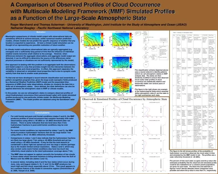
Conclusions • For cold frontal and post-cold frontal conditions (states 5 and 6), the MMF produces profiles of cloud occurrence that compare favorably with radar observations using either a -40 dBZe or -25 dBZe threshold (later not shown). There is some indication that low-level (less than 3 km) hydrometeor fractions in post-cold-frontal conditions may be over predicted. • For warm frontal conditions (as represented by states 1 and 3), the MMF tends to produce hydrometeor fractions that are too large below 7 km using either a -40 or -25 dBZe reflectivity threshold. • Comparisons in states 1 and 3 also indicate that the hydrometeor fractions are likely too large above 7 km using a -40 dBZe threshold and yet too small using a -25 dBZe threshold. It may be that the total amount of condensate is about right but spread out over too large a volume (perhaps due to the models limited vertical resolution). States 2 and 4, which may also contain some warm frontal conditions also have too much low reflectivity cloud relative to the total hydrometeor coverage above 7 km. • The MMF does not appear to capture correctly the formation of low clouds in those states where low-level moisture is being advected from the Gulf of Mexico over the ARM site (states 2 and 12). • In several states, including state 8 and the four states which occur during June, July, and August (states 9, 10, 11 and 12) the MMF produces too much high and thin cloud, especially above 10 km. This result appears to be a common feature of the model in convective regions (Ovtchinnikov et al. 2006, Yunyan et al. 2008). Observed & Simulated Profiles of Cloud Occurrence by Atmospheric State • Motivation • Meaningful comparisons of climate model output with observational data are sometimes difficult to achieve because, unlike numerical weather prediction models, climate models do not predict the specific sequence of weather that any location is expected to experience. At best a climate model simulation can be thought of as representing one possible realization of future weather. • In climate model evaluations observational data are typically aggregated (e.g. averaged) over a sufficiently long period of time that the influence of individual weather events becomes small relative to the average. However, when differences between the aggregate observations and aggregate model output are detected, it can be difficult to determine the source of the differences (what physical processes or situations are not sufficiently represented by the model). • One approach to dealing with this problem is to aggregate both the observations and model output in a way that provides insight into the interaction between the atmospheric state and cloud properties. In effect, this approach separates the variability in observed or simulated cloud properties that is due to synoptic scale activity from that due to smaller scale processes. • To that end we have developed a neural network classification tool (essentially a pattern recognition program) that, given the large-scale (synoptic) fields produced by a Numerical Weather Prediction (NWP) model and the associated time-sequence of ARM cloud radar observations, divides (or clusters) the data into a finite set of atmospheric states. Once defined, the state definitions can also be applied determine the atmospheric state in NWP or climate models. • In this poster, we use our atmospheric states to compare observed profiles of cloud (hydrometeor) occurrence (from ground-based radar) with model simulated profiles produced by one particular climate model, the Multiscale Modeling Framework (MMF). The model profiles are obtained using the Quickbeam radar simulator. A Comparison of Observed Profiles of Cloud Occurrence with Multiscale Modeling Framework (MMF) Simulated Profiles as a Function of the Large-Scale Atmospheric State Roger Marchand and Thomas Ackerman - University of Washington, Joint Institute for the Study of Atmosphere and Ocean (JISAO) Nathaniel Beagley - Pacific Northwest National Laboratory • The classification scheme (depicted above) uses a neural network to identify patterns (which we call atmospheric states) in NWP analysis data. The states are then iteratively modified to ensure that observed (local scale) radar profiles of cloud occurrence are statistically distinct and temporally stable over several years of observations. • The figure to the right shows one example of the meteorological fields which essential define atmospheric state #1 and the table to the right summarizes each state. • The figure to the left shows profiles of the probability of hydrometeor occurrence observed (by cloud radar) in blue and simulated by the MMF model in red. The profiles use a radar reflectivity threshold of –40 dBZe. • The percent of time each state occupies and the p-value (the estimated probability that the observed and simulated profile could be two realizations for a common parent population) are given for each state. The black line and asterisks in figures 4 and 5 denote altitudes where comparison were possible and where the p-value is less than 5%, respectively.