Download
1 / 22
220 likes | 354 Views
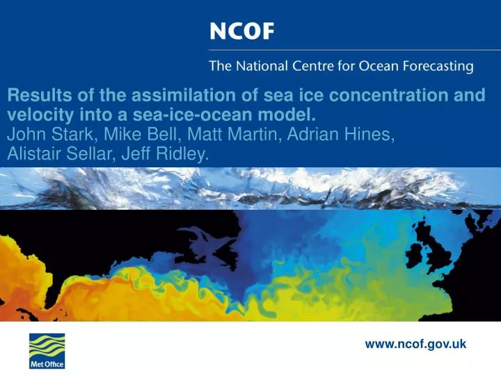
Results of the assimilation of sea ice concentration and velocity into a sea-ice-ocean model. John Stark, Mike Bell, Matt Martin, Adrian Hines, Alistair Sellar, Jeff Ridley. Motivation & Outline of Talk. Motivation Improve operational forecasts of sea-ice and ocean

E N D
Results of the assimilation of sea ice concentration and velocity into a sea-ice-ocean model.John Stark, Mike Bell, Matt Martin, Adrian Hines, Alistair Sellar, Jeff Ridley.
Motivation & Outline of Talk. Motivation • Improve operational forecasts of sea-ice and ocean • Improve seasonal and decadal forecasts • Improve NWP forecasts by using better sea-ice data • Reduce uncertainties in sea-ice models by detailed intercomparison of models & data. Overview of talk • Overview of the assimilation system. • Ice concentration assimilation. • Ice velocity assimilation. • Results from year-long reanalysis integrations • Period from October 1999 December 2000. • Summary
The Sea-Ice-Ocean Model 1° FOAM, Operational since 1997 1° Global FOAM. • Ocean component is identical to the operational FOAM model. • 6-hourly NWP fluxes. • Ice thickness distribution (ITD), 5 categories (Lipscomb 2001). • Elastic viscous plastic rheology (Hunke & Dukowicz 1997) • Derived from the CICE model (Hunke & Lipscomb, LANL) • Configuration of sea ice model is identical to our latest climate model, HadGEM1. • Regular Lat-Long grid (Polar island participates in ice flow)
Sea Ice Concentration Assimilation Scheme ASI algorithm & Q.C. NWP surface temperature Ice concentration • Obs from SSM/I (passive microwave). • ASI algorithm converts brightness temperature to ice concentration estimates. • Optimal interpolation used : • Can process many observations efficiently. • Can cope with poor estimates of the error. • Does not require accurate knowledge of error correlations (but these can be used). • Does not require an adjoint or inverse model or ensemble runs. Forecast O.I. Analysis Swath data Analysis Increments SST & Ice
Observation Pre-Processing • Very large number of observations : more than 300,000 per day. • Sub-sampled to include only observations with all 7 channels (85GHz is sampled at twice the frequency in both directions). • Helps to reduce error correlation, since beam footprint is larger than spatial sampling. • Used a maximum ice extent mask to reduce spurious observations in sub-tropics and reduce the total number of observations. • Land masks extended to 100km Ice extent mask for March
Ice Conc. Observation Pre-Processing • Observations that fail the weather filter are treated as 0% ice cover. Swath Obs, Tb Ice Extent Filter NASA-Team Fail Conc=0% Weather Filter NWP Surface T. Fail Discard NTA > 30% ? Error Estimate Conc(ASI)
Effect of 30% NTA threshold. • Trade off between spurious ice observations & resolving the marginal ice zone: Threshold = 5% Threshold = 30%
Application of Analysis Increments • The analysis scheme provides an estimate of total sea ice concentration • This must be mapped onto the ice thickness distribution (ITD) in the model. • Preferentially altering the thinnest ice. • Smallest change in heat content • Represents thermodynamic changes to the sea ice. • Scaling all categories • Smallest RMS change in category ice area. • Represents convergence / divergence in the flow. • Can result in large changes to thick ice. Fractional Cover Ice Thickness
Application of Analysis Increments Scaling all categories Fractional Cover Red = Free run Cyan = Assim Ice Thickness Fractional Cover Red = Free run Cyan = Assim Ice Thickness
Ice Velocity Assimilation Scheme Obs Q.C. Analysis Analysis increments Balancing stress Computed using free drift i Forecast Ice-motion data from CERSAT-IFREMER and NSIDC Model ice velocity bias Ice motion forecast
Ice Vel. Observation Pre-Processing Fowler Obs (ASCII) CERSAT Obs (NetCDF) Coordinate Conversion & Vector Rotation Fail Discard Quality Flag==1 ? Model N-day Mean Velocities Fail Discard V > 1m/s ? Interpolate to Obs Combine with Ob Errors, output to Obs file.
Velocity analysis scheme • Assimilation • Assimilation scheme based on OI, similar to ice concentration. • Assimilation scheme able to control divergence introduced by the assimilation. • Relative amount of divergence can be controlled. • Uses a ‘balancing stress’ based on free drift dynamics to apply the increments. • Uses 2 background error length scales. • Quality Control • Observations near coastlines have reduced impact to prevent velocities into land.
Ice Velocity : Application of Increments • EVP scheme rapidly adjusts to maintain equilibrium with external forcing on ice. • Direct application of the analysis increments to the velocity fails. • Previous work (Meier, Zhang) has diagnosed an additional velocity which is added to the model and plays no direct part in the dynamics. • We used an alternative approach : balancing stress. Ice velocity after a perturbation compared to a control run.
Ice Velocity : Application of Increments Ice velocity assimilation using a ‘balancing stress’ • An additional term was added to the model sea-ice momentum equation to apply the velocity increments. • The additional stress term is computed by assuming the sea-ice is in free drift. • The first term on the right is the additional stress required to balance the ice-ocean stress, the second term comes from the Coriolis term. • This is a non-linear term since it depends on the sea ice velocity and not just the increment.
Outline of Talk. • Overview of the assimilation system. • Ice concentration assimilation. • Ice velocity assimilation. • Results from year-long reanalysis integrations • Period from October 1999 December 2000. • Summary
Snap Shots : March 1, 2000 After 150 days of assim. Control Conc. Assim. Ice Concentration ASI Gridded. Vel. Assim Conc. & Vel. Assim
Snap Shots : Sept 1, 2000 After 335 days of assim. Control Conc. Assim. Ice Concentration ASI Gridded. Vel. Assim Conc. & Vel. Assim
Ice concentration statistics. • Significant improvement with ice conc. assimilation. • Small difference with ice vel. assimilation. • Melt season a particular problem. 1° Global 1/3° Arctic 1° Global
Velocity Comparison with Buoy Motion • Motion computed offline from 1-day mean model fields. • Assimilation improves representation of buoy motion during winter. Less improvement during summer.
Impact of velocity assim. on thickness. • Velocity assimilation led to changes in thickness of order 30cm. • Thicker ice around Greenland and Fram Strait. • Thinner in Beaufort Gyre. Annual avg. thickness change (m) (assim. – control)
Correlation between velocity increments and wind stress. Zonal Wind / Assim, October 1999 Meridional Wind / Assim, October 1999 Zonal Wind / Assim, March 2000 Meridional Wind / Assim, March 2000 Strong negative correlation in many areas indicates wind stress too strong.
Summary • The ice concentration and velocity assimilation has been shown to give quantitative improvements in modelled sea ice. • Very little coupling between ice concentration and ice velocity in this model. • Ice dynamics has little impact on ice concentration in this model. • Velocity analysis increments applied indirectly, via a balancing stress. • Ice velocity cannot be directly assimilated using an EVP model. • Use of bias correction techniques allows forecast improvement & reduces RMS errors. • Diagnosis of deficiencies in the model and forcing are possible using the assimilation.