Download
1 / 35
350 likes | 420 Views
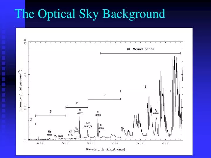
The Optical Sky Background. The Optical Sky. I: the V – I band. The Optical Sky. II: the R - I band. The Optical Sky. III: the I - Z band. The Optical Sky. IV: the z – J band. The Optical Sky. V. The Near-IR Sky Background. The Sky OH Emission Lines. The Sky OH Emission lines.

E N D
The Near-IR Sky The traditional J, H and K bands defined by the atmospheric absorption At some wavelengths, the atmosphere is blocking the radiation. If those wavelengths are crucial, space observations are required
Cosmic Volumes. I • Luminosity function • F(L) = f* • exp(-L/L*) • (L/L*)a • f* ~ 10 -2 to 10 -3 Mpc-3 • L* ~ 1011 to 1012 LO or 1044 to 1045 erg/sec • a ~ -1.0 to -1.2 (optical);-1.4 to –1.8 (UV) • Luminosity density • L = ∫ dL • L • f* • exp(-L/L*) • (L/L*)a ~ L*• f*
Cosmic Volumes. II • Maximum Volume • Vmax = A • ∫ f(z) • dV(z)/dz • z • A ~ survey area • f(z) survey redshift distribution function • Effective Volume: the volume visible to you using a galaxy with luminosity L • Veff(L) = V(L) = A • ∫ f(z; L) • dV(z)/dz • z • When measuring luminosity function: V(L)/ Vmax • Always remember COSMIC VARIANCE
Cosmic Volumes. III • At z = 3 • 1 arcsec ~ 3 kpc (physical) ~ 10.2 kpc (comoving) • 10 arcmin ~ 1.8 Mpc (physical) ~ 7.2 Mpc (comoving) • At z=3, dz ~ 1 • dR(z=3) ~ 500 Mpc • FWHM = 100 Å corresponds to dz = 0.08 or • DR = 40 Mpc
Survey Options • Spectroscopy • Slit or slitless spectroscopy • Objective prism imaging • Photometry (imaging) • Narrow band filters • Tunable filters • A cost-benefit analysis of any survey designed should be done in light of the desired scientific goals to achieve
Emission Line SurveysLecture 3 Mauro Giavalisco Space Telescope Science Institute University of Massachusetts, Amherst1 1From January 2007
Observing Strategies: Slit Spectroscopy • dispersed images of targets through slit or slits. Can be blind or targeted (targets pre-selected according to some selection criteria) • PROs: • High sensitivity • Large radial velocity/redshift coverage • Easy selection of spectral coverage • Easy trade off b/w spectral resolution, sensitivity and coverage • CONs: • Very limited spatial coverage • Data acquisition of medium complexity • Data reduction and analysis of medium complexity • Very costly if large volumes of space need to be covered: cost driven by number of individual slit(s)-mask exposures
Observing Strategies: Slitless Spectroscopy • dispersed images through a dispersive spectral element (prism, grism, grating). Blind surveys • PROs: • Large spatial coverage • Large radial velocity/redshift coverage • Relatively large spectral coverage • Trade off b/w spectral resolution and coverage • Easy data acquisition • CONs: • Low sensitivity (high background) • Complex data reduction and analysis • Some spatial coverage losses due to spectra overlapping • Exposure times longer than slit spectroscopy
Observing Strategies: Narrow-Band Imaging • Photometry or “narrow” band imaging: images through a set of filters selected to measure emission line flux and continuum flux density • PROs: • Large spatial coverage • Spatial mapping of emission line regions • Easy data acquisition • Easy data reduction and analysis • CONs: • Limited spectral (radial velocity/redshift) coverage • Increasing spectral coverage (broader filters) decreases sensitivity • Exposure times longer than slit spectroscopy (but shorter than slitless one) • Accurate measure of continuum costly (several bands needed)
Emission-line surveys • Targeted surveys: “a-priory” knowledge of redshift or radial velocity: • Narrow-band imaging: • Best option if coverage of area of sky required. Examples: • Galaxy cluster, supercluster candidates • Slit spectroscopy: • Best sensitivity. Examples: • Galaxies causing QSO or GRB absorption systems
Strategy of Emission-line surveys • Blind surveys: no “a-priory” knowledge of redshift or radial velocity: • Narrow-band imaging: • Useful if large volume density of sources suspected and if large sensitivity can be achieved. Examples: • Distant galaxy searches • Slitless spectroscopy: • Good option if high sensitivity can be achieved (e.g. from space). Examples: • Distant galaxies searches • Slit spectroscopy: • Good option if very high sensitivity required and small volumes OK (esp. from ground). Examples: • DLA galaxies (redshift can be highly unconstrained) • host galaxies of faded GRBs
Survey Design: Narrow-Band Imaging • Emission line detected as excess flux in in-band images compared to off-band images, which measure continuum flux density (essentially, color selection) • In-band images generally obtained through narrow-band spectral elements (solid-state or Fabry-Perot tunable filters). For broad lines and/or large Wl, medium band elements OK. • Off-band images can be either through narrow-band elements (one required; two preferable) or medium and broad-band ones • Best photometric accuracy reached using multiple narrow-band elements. Usually costly • Final sensitivity of the survey is the ability to detect excess flux, not just S/N in in-band images: need to achieve accurate continuum measure to have sensitivity to lines with weak Wl. • Uncertainty on continuum flux density (due to SED scatter and limited “spectral resolution” of using filters, not just S/N of narrow-band image is crucial, especially for weak Wl
Observational Strategies: How to Choose Filters Matsuda et al.
Narrow-Band Imaging: Blind Surveys Rhoads et al.
Slitless Spectroscopy (space): Blind Surveys Rhoads et al. McCarthy et al. (1999)
Slitless Spectroscopy (space): Blind Surveys Rhoads et al. McCarthy et al. (1999)
Slitless Spectroscopy (space): Blind Surveys McCarthy et al. (1999)
Slitless Spectroscopy (space): Blind Surveys McCarthy et al. (1999)
Slit Spectroscopy: Targeted Surveys DLAs in the spectrum of QSOs McCarthy et al. (1999)
Slit Spectroscopy: Targeted Surveys DLAs in the spectrum of QSOs
Slit Spectroscopy: Targeted Surveys DLAs in the spectrum of QSOs
Slit Spectroscopy: Targeted Surveys DLAs in the spectrum of QSOs
Slit Spectroscopy: Targeted Surveys DLAs in the spectrum of QSOs
Lya Surveys: Early Galaxies • Originally designed to find star-forming galaxies at very high redshifts (Partridge Peebles 1967) • ready my ARAA paper (Giavalisco 2002) • Early surveys essentially unsuccesful • Koo & Kron (1980) • Djorgovski et al. (1985) • Lowenthal et al (1990); Thompson et al. (1995) • First to be found by Lya were (steep spectrum) radio galaxies • Spinrad & Djorgovski 1984a,b; Spinrad et al.\ 1985 • Significant results came with advent of 8-m class telescopes • Rhoads et al. (2000) • Taniguchi et al., Ouchi et al. , Matsuda et al. Shimasaku et al.
Lya Surveys • Today, Lya surveys mostly useful to complement continuum-based searches: • Fainter continuum levels • Trace LSS, clustering, clusters • Spatial mapping of emitting regions • Constraints on reionization