Download
1 / 44
440 likes | 595 Views
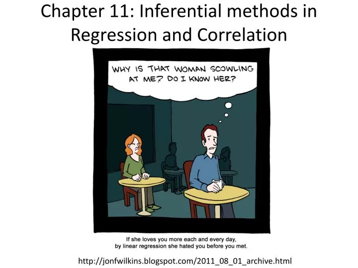
Chapter 11: Inferential methods in Regression and Correlation. http://jonfwilkins.blogspot.com/2011_08_01_archive.html. Example: distribution of y.

E N D
Chapter 11: Inferential methods in Regression and Correlation http://jonfwilkins.blogspot.com/2011_08_01_archive.html
Example: distribution of y The relationship between age and change in systolic blood pressure (BP, mm Hg) after 24 hours in response to a particular treatment has a linear regression equation of y = 20.11 – 0.526x + e with σ = 6.52. • What is the mean value of y when x = 30? x = 50? x = 70? • What is the standard deviation of y when x = 30? x = 50? x = 70?
Example: Estimating and The cetane number is a critical property in specifying the ignition quality of a fuel used in a diesel engine. Determination of this number for a biodiesel fuel is expensive and time-consuming. Therefore a way of predicting this number is wanted. The data on the next slide is x = iodine value (g) and y = cetane number for a sample of 14 biofuels. The iodine value is the amount of iodine necessary to saturate a sample of 100g of oil. • What are the point estimates of and ? • What is a point estimate of the true average cetane number whose iodine value is 100?
Example: Estimating and (cont) What are the point estimates of and ?
Example: Estimating and (cont) b) What is a point estimate of the true average cetane number whose iodine value is 100?
Example: Estimating and The cetane number is a critical property in specifying the ignition quality of a fuel used in a diesel engine. Determination of this number for a biodiesel fuel is expensive and time-consuming. Therefore a way of predicting this number is wanted. The data on the next slide is x = iodine value (g) and y = cetane number for a sample of 14 biofuels. The iodine value is the amount of iodine necessary to saturate a sample of 100g of oil. c) Find the point estimate of the error standard deviation, σ. d) What proportion of the observed variation in y can be attributed to the simple linear regression relationship between x and y?
Example: Estimating and (cont) c) Find the point estimate of the error standard deviation, σ. d) What proportion of the observed variation in y can be attributed to the simple linear regression relationship between x and y?
Example: Estimating and (SAS) The REG Procedure Model: MODEL1 Dependent Variable: cetane Number of Observations Read 15 Number of Observations Used 14 Number of Observations with Missing Values 1 Analysis of Variance Sum of Mean Source DF Squares Square F Value Pr > F Model 1 298.25443 298.25443 45.35 <.0001 Error 12 78.91986 6.57665 Corrected Total 13 377.17429 Root MSE 2.56450 R-Square 0.7908 Dependent Mean 55.65714 Adj R-Sq 0.7733 CoeffVar 4.60767 Parameter Estimates Parameter Standard Variable DF Estimate Error t Value Pr > |t| Intercept 1 75.21243 2.98363 25.21 <.0001 iodine 1 -0.20939 0.03109 -6.73 <.0001
Example: CI The cetane number is a critical property in specifying the ignition quality of a fuel used in a diesel engine. Determination of this number for a biodiesel fuel is expensive and time-consuming. Therefore a way of predicting this number is wanted. The data on the next slide is x = iodine value (g) and y = cetane number for a sample of 14 biofuels. The iodine value is the amount of iodine necessary to saturate a sample of 100g of oil. e) What is the 95% CI for the true slope?
Example: Output (SAS) The SAS System 09:20 Thursday, November 10, 2011 3 The REG Procedure Model: MODEL1 Dependent Variable: cetane Number of Observations Read 15 Number of Observations Used 14 Number of Observations with Missing Values 1 Analysis of Variance Sum of Mean Source DF Squares Square F Value Pr > F Model 1 298.25443 298.25443 45.35 <.0001 Error 12 78.91986 6.57665 Corrected Total 13 377.17429 Root MSE 2.56450 R-Square 0.7908 Dependent Mean 55.65714 Adj R-Sq 0.7733 CoeffVar 4.60767 Parameter Estimates Parameter Standard Variable DF Estimate Error t Value Pr > |t| 95% Confidence Limits Intercept 1 75.21243 2.98363 25.21 <.0001 68.71165 81.71321 iodine 1 -0.20939 0.03109 -6.73 <.0001 -0.27713 -0.14164 Sxx = 6802.7693
Example: Hypothesis test The cetane number is a critical property in specifying the ignition quality of a fuel used in a diesel engine. Determination of this number for a biodiesel fuel is expensive and time-consuming. Therefore a way of predicting this number is wanted. The data on the next slide is x = iodine value (g) and y = cetane number for a sample of 14 biofuels. The iodine value is the amount of iodine necessary to saturate a sample of 100g of oil. f) Is the model useful (that is, is there a useful linear relationship between x and y)?
Example: Hypothesis test (SAS) The REG Procedure Model: MODEL1 Dependent Variable: cetane Number of Observations Read 15 Number of Observations Used 14 Number of Observations with Missing Values 1 Analysis of Variance Sum of Mean Source DF Squares Square F Value Pr > F Model 1 298.25443 298.25443 45.35 <.0001 Error 12 78.91986 6.57665 Corrected Total 13 377.17429 Root MSE 2.56450 R-Square 0.7908 Dependent Mean 55.65714 Adj R-Sq 0.7733 CoeffVar 4.60767 Parameter Estimates Parameter Standard Variable DF Estimate Error t Value Pr > |t| Intercept 1 75.21243 2.98363 25.21 <.0001 iodine 1-0.209390.03109-6.73<.0001
Example: ANOVA (SAS) The REG Procedure Model: MODEL1 Dependent Variable: cetane Number of Observations Read 15 Number of Observations Used 14 Number of Observations with Missing Values 1 Analysis of Variance Sum of Mean Source DF Squares Square F Value Pr > F Model 1 298.25443 298.25443 45.35 <.0001 Error 12 78.91986 6.57665 Corrected Total 13 377.17429 Root MSE 2.56450 R-Square 0.7908 Dependent Mean 55.65714 Adj R-Sq 0.7733 CoeffVar 4.60767 Parameter Estimates Parameter Standard Variable DF Estimate Error t Value Pr > |t| Intercept 1 75.21243 2.98363 25.21 <.0001 iodine 1 -0.20939 0.03109 -6.73 <.0001
Example: Hypothesis test for The cetane number is a critical property in specifying the ignition quality of a fuel used in a diesel engine. Determination of this number for a biodiesel fuel is expensive and time-consuming. Therefore a way of predicting this number is wanted. The data on the next slide is x = iodine value (g) and y = cetane number for a sample of 14 biofuels. The iodine value is the amount of iodine necessary to saturate a sample of 100g of oil. g) Is the model useful (that is, is there a useful linear relationship between x and y) using the population correlation coefficient?
Example: ANOVA (SAS) The REG Procedure Model: MODEL1 Dependent Variable: cetane Number of Observations Read 15 Number of Observations Used 14 Number of Observations with Missing Values 1 Analysis of Variance Sum of Mean Source DF Squares Square F Value Pr > F Model 1 298.25443 298.25443 45.35 <.0001 Error 12 78.91986 6.57665 Corrected Total 13 377.17429 Root MSE 2.56450 R-Square 0.7908 Dependent Mean 55.65714 Adj R-Sq 0.7733 CoeffVar 4.60767 Parameter Estimates Parameter Standard Variable DF Estimate Error t Value Pr > |t| Intercept 1 75.21243 2.98363 25.21 <.0001 iodine 1 -0.20939 0.03109 -6.73<.0001
Example: Hypothesis test for (2) In some locations, there is a strong association between concentrations for two different pollutants. The following data consists of the concentrations of x = ozone (ppm) and y = secondary carbon concentration (μg/m3).
Example: Hypothesis test for (2) The summary statistics are: Using the population correlation coefficient, is this model useful?
Example: Hypothesis test for (2) Analysis of Variance Sum of Mean Source DF Squares Square F Value Pr > F Model 1 222.47934 222.47934 14.69 0.0018 Error 14 212.05816 15.14701 Corrected Total 15 434.53750 Root MSE 3.89192 R-Square 0.5120 Dependent Mean 10.66250 Adj R-Sq 0.4771 CoeffVar 36.50097 Parameter Estimates Parameter Standard Variable DF Estimate Error t Value Pr > |t| Intercept 1 0.99801 2.70292 0.37 0.7175 x 1 93.37670 24.36448 3.83 0.0018
Example: Hypothesis test for (2) The REG Procedure Model: MODEL1 Dependent Variable: cetane Number of Observations Read 15 Number of Observations Used 14 Number of Observations with Missing Values 1 Analysis of Variance Sum of Mean Source DF Squares Square F Value Pr > F Model 1 298.25443 298.25443 45.35 <.0001 Error 12 78.91986 6.57665 Corrected Total 13 377.17429 Root MSE 2.56450 R-Square 0.7908 Dependent Mean 55.65714 Adj R-Sq 0.7733 CoeffVar 4.60767 Parameter Estimates Parameter Standard Variable DF Estimate Error t Value Pr > |t| Intercept 1 75.21243 2.98363 25.21 <.0001 iodine 1 -0.20939 0.03109 -6.73<.0001
Example: Multiple Linear Regression It is important to know how long a tool will last (min) in the industrial setting. The cutting tool in this study is used to cut a particular type and size of cold-rolled steel. The predictors of interest are x1 = cutting speed (feet/min), x2 = feed rate (in/revolution) and x3 = depth of cut (in). The predicted model is y = 101.765 – 0.0958 x1 – 667.972 x2 - 472.304 x3 + e a) What is the mean life of a tool that is being used to cut depths of 0.03 inch at a speed rate of 450 feet/min with a feed rate of 0.01 in/revolution? b) What is the interpretation of 1 = -0.0958? Of 2 = -667.972? Of 3 = -472.304?
Example: Polynomial Regression Suppose the mean daily peak load (MW) for a power plant and the maximum outdoor temperature (oF) for a sample of 10 days is given below. • What is the estimated regression line using a quadratic regression model (besides the equation of the line, include the values of adj. r2 and se? • Using the line, predict the required peak power if the temperature is 98 oF?
Example: Polynomial Regression (SAS) datanewpower; set power; temp2 = temp*temp; procreg data=newpower; model load=temp temp2; output out=fit r=res; run; Analysis of Variance Sum of Mean Source DF Squares Square F Value Pr > F Model 2 18089 9044.26725 53.88 <.0001 Error 7 1175.06549 167.86650 Corrected Total 9 19264 Root MSE 12.95633 R-Square 0.9390 Dependent Mean 194.80000 Adj R-Sq 0.9216 CoeffVar 6.65109 Parameter Estimates Parameter Standard Variable DF Estimate Error t Value Pr > |t| Intercept 1 1784.18833 944.12303 1.89 0.1007 temp 1 -42.38624 21.00079 -2.02 0.0833 temp2 1 0.27216 0.11634 2.34 0.0519
Example: Polynomial Regression (cont) b) Using the line, predict the required peak power if the temperature is 98 oF?
I love statistics! Thank you for not eating me!
Example: Multiple RegressionQualitative Predictors A study is conducted to determine the effects of x1 = company size and x2 = the presence (1) or absence (0) of a safety program on y = the number of work hours lost due to work-related accidents (thousands). 20 companies with no active safety programs were randomly chosen and 20 companies with active safety programs were randomly chosen. The SAS file (qualpred.txt) is on the class notes web site. The estimated regression line is ŷ = 31.6244 + 0.01428 x1 – 58.0779 x2 + e What are the interpretations of 1 = 0.01428 and 2 = -58.0779?
Conceptual Understanding X3 X1 X2 Total Variation of Y
Example: Multiple Linear Regression It is important to know how long a tool will last (min) in the industrial setting. The cutting tool in this study is used to cut a particular type and size of cold-rolled steel. The predictors of interest are x1 = cutting speed (feet/min), x2 = feed rate (in/revolution) and x3 = depth of cut (in). a) Is there a useful linear relationship between the cutting tool lifetime and the predictors?
Example: MLR (cont) Analysis of Variance Sum of Mean Source DF Squares Square F Value Pr > F Model 3 2743.82814 914.60938 20.93<.0001 Error 20 874.13019 43.70651 Corrected Total 23 3617.95833 Root MSE 6.61109 R-Square 0.7584 Dependent Mean 38.54167 Adj R-Sq 0.7222 CoeffVar 17.15310 Parameter Estimates Parameter Standard Variable DF Estimate Error t Value Pr > |t| Intercept 1 101.76536 8.33310 12.21 <.0001 speed 1 -0.09578 0.01426 -6.72 <.0001 feed 1 -667.97241 386.23081 -1.73 0.0991 depth 1 -472.30426 161.81434 -2.92 0.0085
Example: MLR (cont) Analysis of Variance Sum of Mean Source DF Squares Square F Value Pr > F Model 3 2743.82814 914.60938 20.93 <.0001 Error 20 874.13019 43.70651 Corrected Total 23 3617.95833 Root MSE 6.61109 R-Square 0.7584 Dependent Mean 38.54167 Adj R-Sq 0.7222 CoeffVar 17.15310 Parameter Estimates Parameter Standard Variable DF Estimate Error t Value Pr > |t| Intercept 1 101.76536 8.33310 12.21 <.0001 speed 1 -0.09578 0.01426 -6.72 <.0001 feed 1 -667.97241 386.23081 -1.73 0.0991 depth 1 -472.30426 161.81434 -2.92 0.0085
Conceptual Understanding X3 X1 X2 Total Variation of Y
Example: MLR (backwards elimination) Analysis of Variance Sum of Mean Source DF Squares Square F Value Pr > F Model 3 2743.82814 914.60938 20.93 <.0001 Error 20 874.13019 43.70651 Corrected Total 23 3617.95833 Root MSE 6.61109 R-Square 0.7584 Dependent Mean 38.54167 Adj R-Sq 0.7222 CoeffVar 17.15310 Parameter Estimates Parameter Standard Variable DF Estimate Error t Value Pr > |t| Intercept 1 101.76536 8.33310 12.21 <.0001 speed 1 -0.09578 0.01426 -6.72 <.0001 feed 1 -667.97241 386.23081 -1.73 0.0991 depth 1 -472.30426 161.81434 -2.92 0.0085
Example: MLR (backwards elimination) (cont) Analysis of Variance Sum of Mean Source DF Squares Square F Value Pr > F Model 2 2613.09992 1306.54996 27.30 <.0001 Error 21 1004.85841 47.85040 Corrected Total 23 3617.95833 Root MSE 6.91740 R-Square 0.7223 Dependent Mean 38.54167 Adj R-Sq 0.6958 CoeffVar 17.94784 Parameter Estimates Parameter Standard Variable DF Estimate Error t Value Pr > |t| Intercept 1 95.88869 7.96137 12.04 <.0001 speed 1 -0.09543 0.01492 -6.40 <.0001 depth 1 -500.32482 168.46077 -2.97 0.0073