Download
1 / 74
740 likes | 860 Views
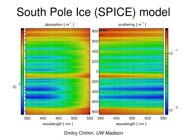
South Pole Ice (SPICE) model. Dmitry Chirkin, UW Madison. Outline. Introduction: experimental setup Improved data processing: new feature extraction New features of/news from ppc Ice anisotropy Improved likelihood description and optimized binning Results. Experimental setup.

E N D
South Pole Ice (SPICE) model Dmitry Chirkin, UW Madison
Outline • Introduction: experimental setup • Improved data processing: new feature extraction • New features of/news from ppc • Ice anisotropy • Improved likelihood description and optimized binning • Results
Updates to the calibration and feature extraction in the fat-reader Fall 2010
waveform baseline • baseline corrections to ATWD0,1,2 and FADC are gathered from the data: • from 0-bin of the waveform • from beacon launches, if available (new) • may change during run (updated in incr*step intervals, e.g., 10 sec) • performed in float numbers (new) from beacons from bin #0 quality cut More plots here: http://icecube.wisc.edu/~dima/work/WISC/nnls/ps/
Timing of DOM launches in DAQ • FADC nominal delay time: 7*25-2.4-75.4-5*3.3=113.7 ns • extra 2 clock cycles for TestDAQ • 1 cycle+15 ns correction to domcal<7.2 values • 15 ns correction to domcal<7.5 values • sign of ATWD1 delta correct, but definition wrong?
Remaining ATWD-FADC offset DAQ testDAQ
Some new features • new implementation of unfolding, based on NNLS (my translation to C of Fortran code by Lawson and Hanson); old Bayesian unfolding still there • adaptive baseline calculation, uses simplified topological trigger logic: • Merge all sets of waveform values that have all of the 7 consecutive samples are within 4.5*[bin size] of each other • fit a line, use to extrapolate baseline (in the vicinity of the fit) • the waveforms are split into non-overlapping non-zero segments that are fed into the unfolding routine. This is very efficient, thus no need to resort to special treatment of simple waveforms. • SLC pulses are unfolded just like any other FADC waveform • for part of FADC overlapping with ATWD the saturated values are recovered by re-convolving the pulses extracted from ATWD. This improves the droop correction of the FADC waveform. • droop is carried-over from the previous DOM launch • across both launches and events • checks that there was not too much droop
Channel merging new Launch #0 Launch #1 old • old: exclusion window after the end of ATWD • new: Subtract FADC SPE-shape-convoluted ATWD pulses from FADC waveform, then combine
Example in flasher data More examples here: http://icecube.wisc.edu/~dima/work/IceCube-ftp/nnls/
Example in flasher data Launch #0 ATWD Launch #0 FADC DOM 64-30, when DOM 63-30 flashing
Example in flasher data Launch #1 ATWD Launch #1 FADC DOM 64-30, when DOM 63-30 flashing
Direct photon tracking with PPC photon propagation code execution threads propagation steps scattering (rotation) photon absorbed GPU scaling: (Graphics Processing Unit) CPU c++: 1.00 1.00 Assembly: 1.25 1.37 GTX 295: 147 157 new photon created (taken from the pool) threads complete their execution (no more photons)
News with PPC • new version: in OpenCL • now written in/for 4 languages/platforms: • c++, Assembly, c for CUDA, c with OpenCL • All of these agree with each other, and with i3mcml • Now confirmed that clsim agrees with ppc as well • better flasher angular distribution • Angular emission profile is specified with 2 rms widths: • vertical=9.7 horizontal=9.8 (tilted LEDs) • vertical=9.2 horizontal=10.1 (horizontal LEDs) • Old: simulated a rectangle in theta, phi with rms given above • New: simulate a 2d Gaussian (von Mises-Fisher distribution) • with the average rms width of 9.7 degrees. • Both are approximations, the 2d Gaussian is probably better. • direct hole ice simulation • anisotropic ice simulation Fall 2011
Direct Hole Ice simulation Hole radius = ½ nominal DOM radius Hole effective scattering ~ 50 cm Hole absorption ~ 100 m Do we need more detailed DOM simulation, including info about both the direction and point on the DOM surface? Perhaps not, if the scattering length in the hole is not much shorter than the hole radius (speculation).
DOM 20,20 20,19: nz=cosh. nominal direct hole ice
enhancement deficit DOM 20,20 20,19: xz nominal hole ice Ratio direct hole ice/nominal
deficit enhancement DOM 20,20 20,21: xz nominal hole ice
remarks • Effect of the hole ice is quite subtle: • The number of photons is reduced on the side facing the emitter, and enhanced in the direction away from the emitter. • The traditional “hole ice” implementation via the angular sensitivity modification reduces the number of photons in the direction into the PMT, and enhances the number of photons arriving into the back of the PMT. • If the emitter is inside the hole ice, the enhancement of photons received on the same string is dramatic. • Either effect is much smaller when receiver is on the different string • can decouple measurement of bulk ice properties from the hole ice
Approximation to Mie scattering Simplified Liu: Henyey-Greenstein: fSL Mie: Describes scattering on acid, mineral, salt, and soot with concentrations and radii at SP Summer 2010
Ice anisotropy? Winter 2011
Evidence in flasher data 53 62 72 71 54 64 70 77 69 45 55 56
What is Ice anisotropy Naïve approximation: multiply the scattering coefficient by a function of photon direction, e.g., by 1 + b ( cos2q - 1/3 ) However, this is unphysical: s(nin,nout) = s(-nout,-nin) (time-reversal symmetry) s(nin,nout) = s(-nin,-nout) (symmetry of ice) s(nin,nout) = s(nout,nin) Direction of less scattering Direction of more scattering
A possible parameterization The scattering function we use is f(cos q), a combination of HG and SL. How about this extension: f(cos q)= f(nin.nout) f(Anin. Anout) a 0 0 A = 0 b 0 in the basis of the 2 scattering axes and z (a,b are, e.g., 1.05). 0 0 1/ab However, function f(cos q) is well-defined for only cos q between -1 and 1. A possible modification is nin Anin/| Anin | nout A-1nout/| A-1nout |. This introduces two extra parameters: a,b (in addition to the direction of scattering preference). The geometric scattering coefficient is constant with azimuth. However, the effective scattering coefficient receives azimuthal dependence as:
Fitting for the anisotropy coefficients k1=0.040, k2=-0.082
Effect of anisotropy on simulation a=1.0 a=1.05, b=0.93
How important is anisotropy? threshold: > 0, 1, 10, 100, 400 p.e. threshold: > 10 p.e. so-so 30% awesome! 21% from SPICE paper
Likelihood description of data: SPICE Mie Sum over emitters, receivers, time bins in receiver Find expectations for data and simulation by minimizing –log of Measured in simulation: s and in data: d; ns and nd: number of simulated and data flasher events Regularization terms:
Likelihood description of data Sum over emitters, receivers, time bins in receiver • Two c2 functions were used: • cq2: sum over total charges only (no time information) ~ 38700 terms • ct2: sum over total charges split in 25-ns bins ~ 2.7.106 terms • Both zero and non-zero contributions contribute to the sum • however, the terms in the above sum are 0 when both d=0 and s=0.
Exact description: new Suppose we repeat the measurement in data nd times and in simulation ns times. The ms and md are the expectation mean values of counts per measurement in simulation and in data. With the total count in the combined set of simulation and data is s + d , the conditional probability distribution function of observing s simulation and d data counts is There is an obvious constraint which can be derived, e.g., from the normalization condition
Two hypotheses: If data data and simulation are unrelated and completely independent from each other, then we can maximize the likelihood for ms and md independently, which with the above constraint yields On the other hand, we can assume that data and simulation come from the same process, i.e., We can compare the two hypotheses by forming a likelihood ratio
Example 2000 200 To enhance the differences between the two likelihood approaches, consider that the amount of simulation is only 1/10th of that of data
Using full range of the data and simulation Simulated exp(-x/5.0) with mean of 5.0