Download
1 / 56
560 likes | 697 Views
Maa-57.2040 Kaukokartoituksen yleiskurssi General Remote Sensing Image enhancement I. Autumn 2007 Markus Törmä Markus.Torma@tkk.fi. Image restoration. Errors due to imaging process are removed Geometric errors position of image pixel is not correct one when compared to ground

E N D
Maa-57.2040 Kaukokartoituksen yleiskurssiGeneral Remote SensingImage enhancement I Autumn 2007 Markus Törmä Markus.Torma@tkk.fi
Image restoration • Errors due to imaging process are removed • Geometric errors • position of image pixel is not correct one when compared to ground • Radiometric errors • measured radiation do not correspond radiation leaving ground • Aim is to form faultless image of scene
Image enhancement • Image is made better suitable for interpretation • Different objects will be seen better manipulation of image contrast and colors • Different features (e.g. linear features) will be seen better e.g. filtering methods • Multispectral images: combination of image channels to compress and enhance imformation • ratio images • image transformations • Necessary information is emphasized, unnecessary removed
Image enhancement • Image is processed to be more suitable for interpretation • Pixel operations: DN of pixel is changed independent to other pixels • sum, multiply, subtract, ratio with constant • Local operations: DN is changed using DN of pixels which are spatially close • filtering • Global operations: all DNs have effect to DN • histogram manipulation • transformation to zero mean and unit deviation
HISTOGRAM • Graphical representation of probability of occurrence of image DNs • Horizontal axis: DN from 0 to 255 • Vertical axis: number of pixels with DN or probability of occurrence of DN in image
HISTOGRAM • DNs of image are usually in narrower region that monitor can show • usually at the darker end of scale • DNs are scaled to larger area more DNs are used from wider region and image interpretation is enhanced
HISTOGRAM • Histogram equalization: scaling is weighted according to probability of occurrence of DNs • More DNs are used to present commonly occurring DNs
HISTOGRAM • Nonlinearly equalized histogram: also other kinds of mathematical functions or combinations of functions can be used • E.g. equalized histogram should be similar to normal distribution
HISTOGRAM • Thresholding: DNs are divided to two groups • DNs less than threshold 0 • DNs more that threshold 1 • E.g. separate water areas from land areas
HISTOGRAM "Level Slicing” • Histogram is divided to levels • considerably less than original DNs • DNs within one level are presented using one grey level or color • Usually used to visualize • thermal images • vegetation index images
HISTOGRAM • Level Slicing: BW and color vesion of vegetation index image
Image filtering • Image f is convolved with filtering mask h g = f * h • Image smoothing / low pass filtering: • noise removal • Image sharpening / high pass filtering: • rapid changes in image function are enhanced
Image filtering Image smoothing • Random errors due to instrument noise and data transmission are removed • Average / mean filtering • Median filtering
Image filtering • Based on use of filtering maks h • Simple averaging filtering mask, size 5x5 pixels: • Averaging filtering mask, size 3x3 pixels:
Image filtering • Principle of convolution • Filtered pixel value:
Image filtering • Original PAN and average filtered image with 3x3 filtering window
Image filtering • Original PAN and average filtered image with 7x7 filtering window
Image filtering Median filtering • DN of pixel is median DN of pixels defined by filtering mask • Take pixels under filtering mask sort from smallest to biggest choose median (the middle one) • Useful if noise consists of single intense spikes (removes them) and edges of areas should be preserved (do not alter them)
Image filtering Median filtering
Image filtering • Original PAN and median filtered image with 3x3 filtering window
Image filtering • Original PAN and median filtered image with 7x7 filtering window
Image filtering • Image averaging corresponds to integration of image function • If changes in image function are of interest derivate image function • Image 2-dimensional function: partial derivates in x- and y-direction • Partial derivates are used to determine amount and direction of change in each pixel • In practice derivates are approximated by differences of neighboring pixels • These can also be implemented using filtering masks
Image filtering • Derivative of image function in horizontal direction can be computed using mask:
Image filtering • Derivative of image function in vertical direction can be computed using mask:
Image filtering • Absolute values of partial derivative images...
Image filtering • …here magnitude of derivative is approximated by mean of partial derivatives
Image texture • Spatial variation of image grey levels or colors • Determines smoothness or coarseness of image • Different targets have different texture can help in interpretation • E.g. Spot panchromatic image: • residential area: lots of variations • water: very little variations • coniferous forest: some variations
Image texture • Compute features which describes properties of texture • new images • In most simple case compute average value and deviation of some neighborhood • statistical properties of texture • Some methods can take direction etc. into account • Haralick’s grey level co-occurrence matrix
Image texture • Variance and skewness of distribution, 7x7 window
Multispectral images • Essential information from image channels • All channels are not necessarily useful • do not use if do not need • Some alternatives • ratio images • difference images • index images • image transformations
Visual interpretation • Channelwise Black-and-White image OR • 3 channels at time, color image
Landsat-7 ETM, 29.7.2000: Visible channels blue, green, red Infrared channels
Color image • Humans can distinguish about 20 – 30 grey levels • Usually images have 256 grey levels • it is not possible to distinguish small details • Humans can distinguish millions of colors • should be exploited in interpretation • Computers have additive color system • primary colors are Red, Green and Blue • RGB-system • channels are presented in combination of 3 channels • if reflectance of target is larger in one channel than others, target is colored with that primary color
True color image • Channels are presented using ttheir natural colors: • blue channel using blue primary color • green channel using green primary color • red channel using red primary color • Is possible with instruments with these three channels, like Landsat ETM
False color image • Channels with wavelenghts which humans do not use or visible channels in wrong order • E.g.: • green channel using blue primary color • red channel using green primary color • NIR channel using red primary color
IHS-color coordinates • RGB-color coordinate system is not the only one • IHS: • Intensity: brightness of color • Hue: wavelenght of color • Saturation: purity or greyness of color • Sometimes in order to enhance some feature, make transformation RGB IHS, edit / process image and make transformation IHS RGB • E.g. colors to DEM • 3-channel image: RGB IHS • Change: put DEM to intensity • Make IHS RGB
IHS-color coordinates • Porvoo: ETM 321 and Intensity
IHS-color coordinates • Porvoo: ETM 321 and Hue
IHS-color coordinates • Porvoo: ETM 321 and Saturation
Ratio images • Channel A pixel value is divided by channel B pixel value • E.g. NIR / RED • Emphasizes the differences between channels • Increase difference between vegetated and non-vegetated areas • Images taken at different times changes
Ratio images • If reflectances from different targets are different, channel ratio can emphasize this difference • E.g. Water has low reflectance at near-infrared, bigger at red • Vegetation has low reflectance at red wavelenght, considerably bigger at near-infrared • NIR/PUN: • Very small for water << 1 • Large for vegetation >> 1
Ratio images • Multiplicative factors, which affect all channels, are removed • Effect of topography, sun angle, shadows • Idea is to decrease the variation of DNs of pixels belonging to same land cover • Example: CH1 CH 2 CH1/CH 2 Deciduous forest: • sun 48 50 0.96 • shadow 18 19 0.95 Coniferous forest: • sun 31 45 0.69 • shadow 11 16 0.69
Ratio images • Is vegetation in good or bad condition • NIR/RED higher for vegetation is good condition • As plant becomes ill or autunm comes • Less chlorophyll • Higher reflectance at RED wavelenghts due to smaller chlorophyll absorption • NIR/RED smaller
Ratio images • Ratio images can be more complicated: (CHA - CHB) / (CHC - CHB) • It is wanted to remove some noise or atmospheric effect visible at channel B from channel ratio Problem • In some cases different targets may look the same when their actual reflectances differ • Can be avoided by interpreting ratio images together with some original image channels
OIF: optimum index factor • It is easy to compute many ratio images • Which are best? • Multispectral image, n channels: n(n-1) ratio images • Visual comparison of all combinations takes time • OIF: best combination of three ratio images • Compute image variances and correlations between images • Large variance: good information content • Large correlation between images: images are very much alike • Choose three images, which • Maximize variance • Minimize correlation
Ratio image: example • TM7 (2.2 m) / TM1 (0.48 m): sandy areas white • TM 1.9.1990
Ratio image: example • ETM 29.1.1999
Ratio image: example Changes • Green: more sand 1990 • Red: more sand 1999 • NOTE: Images have been taken at different seasons, so changes might be due to seasonal effects like changes in vegetation or soil moisture
Difference image • Pixel value of channel A is subtracted from channel B value • Image taken at time A is subtracted from image taken at time B • Changes between images • Average filtered image is subtracted from original image • Enhances edges