Download
1 / 17
170 likes | 188 Views
Model A model is a simplified representation of a system at some particular point in time or space intended to promote understanding of the real system. Simulation

E N D
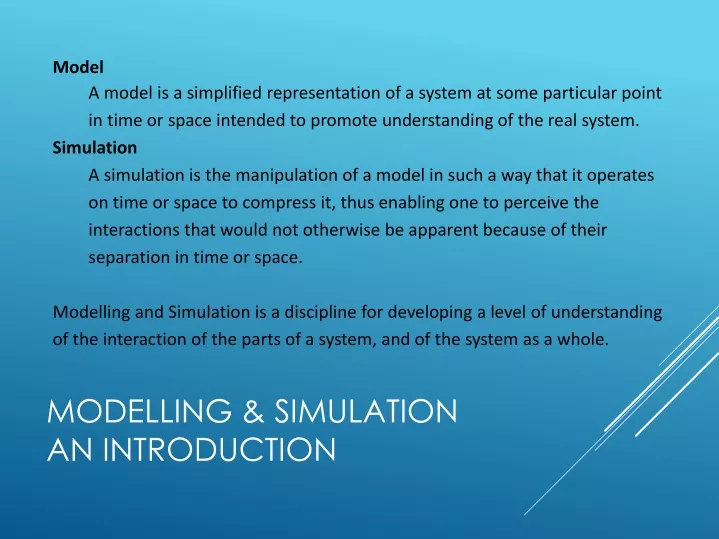
Model A model is a simplified representation of a system at some particular point in time or space intended to promote understanding of the real system. Simulation A simulation is the manipulation of a model in such a way that it operates on time or space to compress it, thus enabling one to perceive the interactions that would not otherwise be apparent because of their separation in time or space. Modelling and Simulation is a discipline for developing a level of understanding of the interaction of the parts of a system, and of the system as a whole. Modelling & SimulationAn Introduction
A simple introduction to numerically modelling the behaviour of a geophysical fluid. THE EFFECTS OF GRAVITY, ROTATION AND SPHERICITY (Scripts and slides adapted from Dr Natalie Burls with acknowledgements to the 2008 ACCESS modelling workshop) Matlab Shallow Water Model A Quick (BUT FUN?!) Tutorial
OR IN MATLAB CODE: % Du/Dt = (f0 + beta*y)v - g*Deta/Dx % Dv/Dt = -(f0 + beta*y)u - g*Deta/Dy % Deta/Dt = -H*(Du/Dx + Dv/Dy) Can be derived from primitive equations based on a number of assumptions: 1) The fluid is barotropic 2) The hydrostatic or shallow water assumption based on H<<L 3) Boussinesq assumption 4) neglect vertical component of Coriolis term 5) neglect small advection and diffusion terms 6) eta << H Shallow Water Equations
OR IN MATLAB CODE: % Du/Dt = (f0 + beta*y)v - g*Deta/Dx % Dv/Dt = -(f0 + beta*y)u - g*Deta/Dy % Deta/Dt = -H*(Du/Dx + Dv/Dy) Can be derived from primitive equations based on a number of assumptions: 1) The fluid is barotropic (density is a function of pressure only) 2) The hydrostatic or shallow water assumption based on H<<L 3) Boussinesq assumption (buoyancy, gravity and turbulence) 4) neglect vertical component of Coriolis term 5) neglect small advection and diffusion terms 6) eta (sea-level height above or below the mean) << H Shallow Water Equations In essence F = ma and conservation of mass are the two physical laws governing this set of equations.
We will run a simple Matlab script which solves the above equations • You will be able to choose: • SIMULATION DURATION (number of days) • BASIN DIMENSIONS (how big or small) • CORIOLIS PARAMETER (spinny spin spin!) • INITIAL PERTURBATION (rock or tsunami) • BATHYMETRY (undersea hole/peak/continental shelf) • PERSPECTIVE (birds-eye view or 3D view) AN OVERVIEW OF THE CODE
Using our simple model we will be simulating the response of a shallow body of water (pond or ocean) to a perturbation to its surface (i.e. dropping a stone into it). In the first example we will neglect the effect of the earths rotation and concentrate only on the effects of gravity. Then in the second example we will add the effects of the earths rotation (Coriolis acceleration – f plane) and observe the change in the response. Finally we will investigate the fact that in reality the magnitude of Coriolis acceleration changes with latitude due to the sphericity of the earth (Beta plane). The effects of gravity, rotation and sphericity
Enter the simulation duration in days • 2 • Enter dimensions of basin in square brackets: • [length(km) width(km) depth(km)] • [10000 10000 1] • Enter 0 for no rotation • Enter 2 for Gaussian hump (2D "bump") • Define diameter of initial perturbation in km • 1000 • Define amplitude of initial perturbation in m • 1 • Bottom topography Enter 0 for flat floor • What type of perspective? You choose 0 or 1 Non Rotating Planet: Exercise 1
Enter the simulation duration in days • same • Enter dimensions of basin in square brackets: • [length(km) width(km) depth(km)] • same • Enter 0 for no rotation • Enter 1 for zonal Gaussian trough (long wave) • Define diameter of initial perturbation in km • same • Define amplitude of initial perturbation in m • same • Bottom topography Enter 0 for flat floor • What type of perspective? You choose 0 or 1 Non Rotating Planet: Exercise 2
Enter the simulation duration in days • same • Enter dimensions of basin in square brackets: • [length(km) width(km) depth(km)] • same • Enter 0 for no rotation • Enter 1 for zonal Gaussian trough (long wave) • Define diameter of initial perturbation in km • same • Define amplitude of initial perturbation in m • same • Bottom topography: Add a ledge! • What type of perspective? You choose 0 or 1 Non Rotating Planet: Exercise 3
Enter the simulation duration in days • same • Enter dimensions of basin in square brackets: • [length(km) width(km) depth(km)] • same • Enter 1 for rotation • Enter 2 for Gaussian hump (2D "bump") • Define diameter of initial perturbation in km • same • Define amplitude of initial perturbation in m • same • Bottom topography Enter 0 for flat floor • What type of perspective? You choose 0 or 1 ADDING ROTATION: Exercise 4 Now play around with perturbation and topography
Agulhas rings depicted in the layer thickness (m) derived from altimeter data (T/P+ERS) and WOA98 hydrographic data during September 26, 1999 http://www-aviso.cnes.fr:8090/HTML/information/publication/news/news8/obrien_fr.html
Enter the simulation duration in days • 5 • Enter dimensions of basin in square brackets: • [length(km) width(km) depth(km)] • same • Enter 2 for beta plane (f changing with latitude) • Enter 2 for Gaussian hump (2D "bump") • Define diameter of initial perturbation in km • 1000 • Define amplitude of initial perturbation in m • 1 • Bottom topography Enter 0 for flat floor • What type of perspective? You choose 0 or 1 Effect of Sphericity: Exercise 5
Enter the simulation duration in days • 5 • Enter dimensions of basin in square brackets: • [length(km) width(km) depth(km)] • same • Enter 3 for beta plane (crossing the equator) • Enter 1 for zonal Gaussian trough (long wave) • Define diameter of initial perturbation in km • 1000 • Define amplitude of initial perturbation in m • 1 • Bottom topography Enter 0 for flat floor • What type of perspective? You choose 0 or 1 Effect of Sphericity: Exercise 6
Mean dynamic topography - oceanic relief corresponding to permanent ocean circulation, computed from hydrologic and drifting buoys, used jointly with altimetry measurements and gravimetric satellite data. Arrows proportional to current speed. This dynamic topography shows all the features of general circulation: gyres and western boundary current (Gulf Stream, Kuroshio, Brazil/Malvinas Confluence area) appear clearly on the map; so too does the Antarctic Circumpolar Current. http://www.aviso.oceanobs.com/en/news/idm/2003/feb-2003-ocean-currents/index.html
TOPEX/Poseidon was the first space mission that allowed scientists to map ocean topography with sufficient accuracy to study the large-scale current systems of the world's ocean. This image was constructed from 10 days of TOPEX/Poseidon data (October 3 to October 12, 1992), yet it reveals most of the current systems identified by shipboard observations collected over the last 100 years. http://en.wikipedia.org/wiki/Ocean_surface_topography