Download
1 / 47
500 likes | 537 Views
GIS, Hydrology and Terrain Analysis Using Digital Elevation Models. David G. Tarboton dtarb@cc.usu.edu. http://www.engineering.usu.edu/dtarb. Overview. GIS as a tool for Hydrologic Modeling The ArcGIS Hydrology Model

E N D
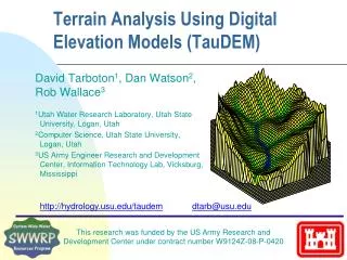
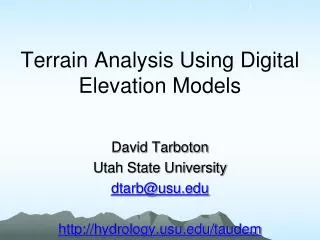
GIS, Hydrology and Terrain Analysis Using Digital Elevation Models David G. Tarboton dtarb@cc.usu.edu http://www.engineering.usu.edu/dtarb
Overview • GIS as a tool for Hydrologic Modeling • The ArcGIS Hydrology Model • Terrain Analysis Using Digital Elevation Models. (Some new Spatial Concepts) • Extendability of ArcGIS (TauDEM as an example) • Demonstration of TauDEM
TOPNET Model Grey River, New Zealand South Island Basin Area: 3817 km2 Flow: 12.1 x 10⁹ m3 Flow/Area: 3184 mm Greymouth Christchurch Subwatershed attributes Stream segment attributes "Data based on contours supplied by Land Information New Zealand"
Spatially constant Parameters Spatially variable Hydraulic conductivity K, calibrated using multiplying factor applied to spatially variable values. The soil capacity parameter ‘soilc’ is estimated as (soil zone depth)/(dth1+dth2)
Basin average precipitation Streamflow at outlet Cumulativewater balance
“White space” is the Grey at Dobson minus Ahaura, Arnold and Grey at Waipuna
SINMAP Terrain Stability Mapping
ArcView Digital Elevation Model ArcView Flood plain maps HEC-RAS Water surface profiles HEC-HMS Flood discharge Flood Plain Mapping CRWR-PrePro AvRAS Digital Map Database Slide from David Maidment, University of Texas at Austin.
HMS Schematic Prepared with CRWR-PrePro Mansfield Dam Colorado River Slide from David Maidment, University of Texas at Austin.
HMS Results Watershed 155 Junction 44 Slide from David Maidment, University of Texas at Austin.
Map-Based Surface Water Runoff Estimating the surface water yield by using a rainfall-runoff function Runoff, Q (mm/yr) Q P Runoff Coefficient C = Q/P Accumulated Runoff (cfs) Precipitation, P (mm/yr) Slide from David Maidment, University of Texas at Austin.
Water Quality: Pollution Loading Module Load [Mass/Time]=Runoff [Vol/Time]x Concentration [Mass/Vol] Precip. Runoff DEM LandUse Accumulated Load EMC Table Load Concentration Slide from David Maidment, University of Texas at Austin.
Bringing together these two communities by using a common geospatial data model http://www.crwr.utexas.edu/giswr GIS Water Resources CRWR GIS in Water Resources Consortium Slide from David Maidment, University of Texas at Austin.
ArcGIS Data Models • Facilitate a process with the user community • Capture the essential, common data model for each discipline • Build a database design template that works well with ArcGIS • Build on experience, not a standards exercise • Share the model on ArcOnline http://arconline.esri.com/arconline/datamodels.cfm Slide from David Maidment, University of Texas at Austin.
Organization B Organization A Organization D Somethingin common Organization C The data model for a business organization tends not to change greatly over time unless the business organization changes the fundamental way that it does business Essential Data Model Slide from David Maidment, University of Texas at Austin.
Flow Time Time Series ArcGIS Hydro Data Model Network Drainage HydroFeatures Hydrography Channel Slide from David Maidment, University of Texas at Austin.
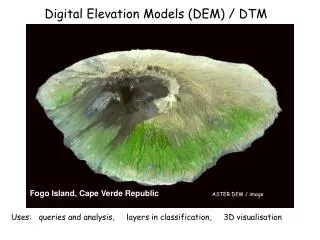
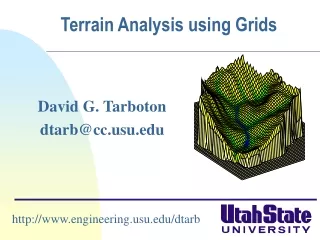
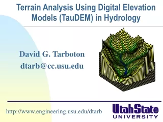
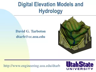
Terrain Analysis Using Digital Elevation Models Elevation Surface — the ground surface elevation at each point Digital Elevation Model — A digital representation of an elevation surface. Examples include a (square) digital elevation grid, triangular irregular network, set of digital line graph contours or random points.
Digital Elevation Grid — a grid of cells (square or rectangular) in some coordinate system having land surface elevation as the value stored in each cell. Square Digital Elevation Grid — a common special case of the digital elevation grid
Digital Elevation Model Based Flow Path Analysis 4 3 2 1 1 1 1 1 5 6 7 1 1 4 3 3 1 8 1 2 1 1 12 Drainage Area 1 1 1 2 16 2 1 3 6 25 D Eight direction pour point model D8 Grid network
? Topographic Slope Topographic Definition Drop/Distance Limitation imposed by 8 grid directions. Flow Direction Field — if the elevation surface is differentiable (except perhaps for countable discontinuities) the horizontal component of the surface normal defines a flow direction field.
The D Algorithm D Flow Direction Grid— A special case of a multiple flow direction grid in which the flow direction is represented by an angle stored in each grid cell Tarboton, D. G., (1997), "A New Method for the Determination of Flow Directions and Contributing Areas in Grid Digital Elevation Models," Water Resources Research, 33(2): 309-319.) (http://www.engineering.usu.edu/cee/faculty/dtarb/dinf.pdf)
Contributing Area using D Contributing Area using D8
Useful for example to track where sediment or contaminant moves
Useful for example to track where a contaminant may come from
Reverse Accumulation Useful for destabilization sensitivity in landslide hazard assessment
Transport limited accumulation Useful for modeling erosion and sediment delivery, the spatial dependence of sediment delivery ratio and contaminant that adheres to sediment
Drainage area can be concentrated or dispersed (specific catchment area)
Stream line Contour line Upslope contributing area a Topographic Definition Specific catchment areaa is the upslope area per unit contour length [m2/m m]
Contributing Area — a field representing at each point the magnitude of the drainage area upslope of that point. Also called Catchment Area, Drainage Area or Flow Accumulation. • Specific Catchment Area — a field representing contributing area per unit contour width. Units are length. • Concentrated Contributing Area — the contributing area on a smooth surface or flow line where surface flow has concentrated and there is a measurable contributing area to a point. Units are area. • Contributing Area Grid — a grid derived from the flow direction grid, which counts in each cell the number of upstream cells draining through that cell.
Hydrologic processes are different on hillslopes and in channels. It is important to recognize this and delineate model elements that account for this. • Concentrated versus dispersed flow. • Objective delineation of channel networks using digital elevation models.
How to decide on drainage area threshold to determine channels and watershed model elements? 500 cell theshold 1000 cell theshold
Same scale, 20 m contour interval Driftwood, PA Sunland, CA Topographic Texture and Drainage Density
Nodes Links Single Stream Strahler Stream OrderStream Drop: Elevation difference between ends of stream • most upstream is order 1 • when two streams of a order i join, a stream of order i+1 is created • when a stream of order i joins a stream of order i+1, stream order is unaltered Note that a “Strahler stream” comprises a sequence of links (reaches or segments) of the same order
Look for statistically significant break in constant stream drop property Break in slope versus contributing area relationship Physical basis in the form instability theory of Smith and Bretherton (1972), see Tarboton et al. 1992 Suggestion: Map channel networks from the DEM at the finest resolution consistent with observed channel network geomorphology ‘laws’.
Statistical Analysis of Stream Drops Threshold = 20 Dd = 1.9 t = -1.03 Threshold = 10 Dd = 2.5 t = -3.5 Threshold = 15 Dd = 2.1 t = -2.08 Stream drop test for Mawheraiti River. For each upward curved support area threshold the stream drop for each stream is plotted against Strahler stream order. The large circles indicate mean stream drop for each order The weighted support area threshold, drainage density (in km-1) and t statistic for the difference in means between lowest order and all higher order streams is given.
Curvature based stream delineation with threshold by constant drop analysis
TauDEM Software Functionality • Pit removal (standard flooding approach) • Flow directions and slope • D8 (standard) • D (Tarboton, 1997, WRR 33(2):309) • Flat routing (Garbrecht and Martz, 1997, JOH 193:204) • Drainage area (D8 and D) • Network and watershed delineation • Support area threshold/channel maintenance coefficient (Standard) • Combined area-slope threshold (Montgomery and Dietrich, 1992, Science, 255:826) • Local curvature based (using Peuker and Douglas, 1975, Comput. Graphics Image Proc. 4:375) • Threshold/drainage density selection by stream drop analysis (Tarboton et al., 1991, Hyd. Proc. 5(1):81) • Wetness index and distance to streams
TauDEM Software Architecture ESRI ArcGIS 8.1 (Toolbar under development ) VB GUI application Standalone command line applications C++ COM DLL interface Available from TauDEM C++ library Fortran (legacy) components http://www.engineering.usu.edu/dtarb/ USU TMDLtoolkit modules (grid, shape, image, dbf, map, mapwin) ESRI gridio API (Spatial analyst) Vector shape files ASCII text grid Binary direct access grid ESRI binary grid Data formats
Implementation Details Spatial Analyst includes a C programming API (Application Programming Interface) that allows you to read and write ESRI grid data sets directly. Excerpt from gioapi.h / * GetWindowCell - Get a cell within the window for a layer, * Client must interpret the type of the output 32 Bit Ptr * to be the type of the layer being read from. * * PutWindowCell - Put a cell within the window for a layer. * Client must ensure that the type of the input 32 Bit Ptr * is the type of the layer being read from. * */ int GetWindowCell(int channel, int rescol, int resrow, CELLTYPE *cell); int PutWindowCell(int channel, int col, int row, CELLTYPE cell);
C++ COM Methods used to implement functionality using Microsoft Visual C++ STDMETHODIMP CtkTauDEM::Areadinf(BSTR angfile, BSTR scafile, long x, long y, int doall, BSTR wfile, int usew, int contcheck, long *result) { USES_CONVERSION; //needed to convert from BSTR to Char* or String *result = area( OLE2A(angfile), OLE2A(scafile), x,y,doall, OLE2A(wfile), usew, contcheck); return S_OK; }
Visual Basic for the GUI and ArcGIS linkage Private TarDEM As New tkTauDEM … Private Function runareadinf(Optional toadd As Boolean = False) As Boolean Dim i As Long runareadinf = False i = TarDEM.Areadinf(tdfiles.ang, tdfiles.sca, 0, 0, 1, "", 0, 1) If TDerror(i) Then Exit Function If toadd Then AddMap tdfiles.sca, 8 End If runareadinf = True End Function
GIS in Water Resources Online A Virtual Course Presented On-Line by David Maidment at the University of Texas at Austin in partnership with Utah State University. Next offering Fall 2002. Goals: • To teach the principles and operation of geographic information systems, focusing in particular on ArcView and its Spatial Analyst extension. • To show how spatial hydrologic modeling can be done by developing a digital representation of the environment in the GIS, then adding functions simulating hydrologic processes. • To develop individual experience in the use of GIS in Water Resources through execution of a term project, and presenting it both orally and written form in html on the world wide web. http://moose.cee.usu.edu/giswr/