Download

1 / 24
250 likes | 297 Views
Multi Function Quine-McCluskey 2-Level Minimization. Shantanu Dutt University of Illinois at Chicago. Acknowledgement: Transcribed to Powerpoint by Huan Ren from Prof. Shantanu Dutt’s handwritten notes. Multiple Output Q-M. General digital system:. Multiple i/p’s. Multiple o/p’s.

E N D
Multi Function Quine-McCluskey 2-Level Minimization Shantanu Dutt University of Illinois at Chicago Acknowledgement: Transcribed to Powerpoint by Huan Ren from Prof. Shantanu Dutt’s handwritten notes
Multiple Output Q-M • General digital system: Multiple i/p’s Multiple o/p’s Share gates as much as possible to reduce cost Sometimes sharing reduces cost; however indiscriminate sharing (e.g., having canonical SOPs for all functions) can actually increase cost. Q: How to do this optimally or near-optimally? A: Multi-function Q-M is one such technique.
α α β β BD α Multiple Output Q-M AB Example 1: CD 00 01 11 10 AD 00 0 4 12 81 α β AD 01 11 51 131 91 β α α β • Separate consideration 11 31 71 111 α α 151 β AB 10 2 6 14 101 β β A fα D ABD α B β D No common implicants used → Total cost =12 [six 2-i/p gates] → 12*2=24 transistors B fβ A A D
Multiple Output Q-M 4 trans. • Example 1 (contd): Now consider common implicants—PIs of the function fa.fb—for inclusion first in each function: • Total cost = • Total literals in distinct/different implicants + total # of implicants (for the 2nd term a common impl. occurring multiple times is counted as many times as it occurs) over all functions = (2+2+3)+4=11 22 transistors (8% cost reduction from separate consideration of the 2 functions) A 4 trans. D fα 6 trans. A B 4 trans. D 4 trans. fβ A B
Multiple Output Q-M α α β β ABD BD α α β CD β X X β β AB Example 2: CD 00 01 11 10 ACD β ABC 00 0 41 121 81 α α β β 01 1 51 131 9 α 11 11 31 71 α α 151 ACD α 10 2 6x 141 10 AB • Taken separately β β β Total cost=18
Multiple Output Q-M (contd.) • Example 2 (contd): Use heuristic “Always include common implicants” Total cost= 14+6=20 (11% cost increase using the above heuristic, from separate consideration of the 2 functions) So how do we determine optimally when and when not to include a common term in an expression ? This can be achieved by the multiple-function QM method.
Multiple-function QM • Difference with single function QM (1) Each minterm is tagged by “flag(s)” of the function it is in. (2) For PI formation, the impl./min-term list is formed for all min-terms/DCs simultaneouslyover all functions. (3) Two impl’s (incl. minterms) can be combined only if they contain same common flags. The new impl. formed by this combining is flagged by the set of common (intersecting) flags. (4) An impl. i that was combined to form a larger impl. can be “checked” (i.e., covered) only if the combined impl. contains all the flags that i contains. In other words, an implicant is covered in the multi-function context if it is covered in each func. that it is an implicant in. (5) In the PIT, the cols are separated by functions, and each minterm for a function is listed under its function’s group—thus a minterm will have separate cols for each function it belongs to. (6) In the PIT, each PI covers minterms only for functions whose flags it contains.
Multiple-function QM (contd.) • All other rules of PIT reduction applies, including the heuristic rules for cyclic PITs (further clarification & caveats given later). Back to Example 1
*a,b 5 5 5 5 5 * * 3 4 bC 2 2 1 1 1 2 1 2 2 1 • PI table: When incl. a multi-func. PI, mark the * w/ only the flags for which it is included More Rules: Rule 5: The row cov. rules (1 and 1’) & cycle-breaking rules 3, 4 apply across the entire PIT, not just in the sub-PIT corresponding to each function. However, the col. cov. rule applies only within the sub-PIT corresp. to a single function (has to do w/ Rule 6 below, as a PI covering a covered col MTi will not necessarily be used to cover the covering col MTj as now there is an extra cost of 1 to do so, and a covering of MTj may be obtained by another PI at a cost of 0 for MTj (e.g., by a p-EPI of MTj’s function that becomes a p-EPI due to another MT in that function) Rule 6: The EPI/pseudo-EPI defn. also applies to only single functions, and if a multi-function PI g is an EPI for some funcs and not for all for which it is an impl, it is only chosen for the former function(s) and not right away for the latter. After this partial inclusion (for some funcs), g’s cost is reduced to 1, and it maybe chosen later for other functions based on this reduced cost. This reduced cost of 1 is not changed any more after future inclusions. The reduction in cost corresponds to the AND gate cost of g which has already been incurred. The remaining cost of 1 corresponds to the OR gate cost in each remaining function for which it may be included later. Note: We will provide an alternative for rule (6) in which an EPI/pseudo-EPI for one func. is also automatically included in all other funcs for which it is an implicant. This alternative uses a sweep-up phase. (same good soln. of cost 11 obtnd. via the include all common impl. heuristic. Note that the bad cover still leads to optimality.)
Rule 6: The EPI/pseudo-EPI defn. also applies to only single functions, and if a multi-function PI g is an EPI for some funcs and not for all for which it is an impl, it is only chosen for the former function(s) and not right away for the latter. After this partial inclusion (for some funcs), g’s cost is reduced to 1, and it maybe chosen later for other functions based on this reduced cost. This reduced cost of 1 is not changed any more after future inclusions. The reduction in cost corresponds to the AND gate cost of g which has already been incurred. The remaining cost of 1 corresponds to the OR gate cost in each remaining function for which it may be included later. Rationale: Minterms p-EPI (@ iter. i) a PIs a a a, b gC @ i+1 a a, b p-EPI (@ i+1) p-EPI for b (@ iteration i-1). Finally, not needed for a. Rule 6 saves a cost of 1 & extra fanout delay for the corresponding gate
* * * gC gC * * 4 1 1 2 2 2 3 5 3 5 6 5 5 7 7 7 1 3 Total cost =13+5=18 Not the bad soln. of cost 20 obtained via the include-all-common-implicants heuristic. Here it was more expensive to include any common implicant, and so none were incuded by multi-QM
α α α α β β β β Example 3 A=0 A=1 BC BC DE 00 01 11 10 DE 00 01 11 10 00 0 41 121 8 00 16 20 28 24 α β 01 01 1 51 131 91 17 211 291 25 α β β 11 11 3 71 11 191 231 151 α α 311 271 α α 10 2 61 141 10 10 18 221 301 26 α α β β ABC ACE ABC ABDE α α α CDE ADE β β α β PI1 PI2 PI3 PI6 PI7 PI4 CDE α PI5
* β 1 α * * * gC * * 4 5 1 3 1 2 2 3 4 7 5 8 6 8 4 5 6 6 4 Total cost=26 • Taking # of MTs covered and cost into consideration Note: For every choice of a multi-func PI g as an EPI/pseudo-EPI for a function, mark each inclusion choice of g by the flag of the function(s) for which it is an EPI/pseudo-EPI (update w/ additional flags as it is included again in more functions). At the end, the flags will determine which functions g should be included in
Three Output Function Example Example 4:
β β a
γ α C 2 5 1 1 2 4 5 3 3 1 3 2 Do QM w/o Rule 6 for PI5 only (Rule 6 used for other multi-function EPI or pseudo-EPI PIs) γ New cost = 1 α,b γ β γ β γ β
γ γ C bC α New cost = 1 1 3 2 2 4 4 5 6 Reduced PIT Total cost = (4+4+5) + (3+1) + (1+4+1) = 23 Note that because of Rule 6, P13 was not unnecessarily included in fb, thus saving a cost of 1. A B C D γ γ β PI1 γ fα PI2 Bad covering but no choice. However, if we consider the two PIs PI9 and PI7 together that PI13 covers, then covering them together is a good covering (cost of 4+1+1 = 6 of PI13 included in fa and fg vs. cost of 3+1 + 3+1 = 8 of incl. PI9 & PI7, resp. in these functions). Thus covering them individually also leads to an optimal soln. in this case (since a good covering of PI13 of {PI9, PI7} exists). This situation also occurred in an earlier example. PI3 fβ PI5 fγ PI13
α,g α α 3 5 4 8 8 7 1 1 7 2 2 2 3 1 9 7 6 Redo Example 4 w/ Rule 6 applied to all multi-function PIs New cost = 1 Pseudo-singleton cols New cost = 1 γ β γ β γ β
Reduced PIT α,g 10 10 3 1 2 3 3 Total cost = (4+4+5) + (3+5) + (1+4+1) = 27 bC Once again, because of Rule 6, we avoid unnecessarily including P13 in fb, and P10 in fa . However due to a combination of Rule 6 and bad covering, PI2 and PI5 not not included in fg and in fb , respectivly, and PI10 of higher total cost than that of PI2 and PI5 used instead. So cost increases by 4+1+1 (cost of PI10 in 2 funcs) – 2 (OR cost of PI5 and PI2, if they were shared) = 4. Total cost = 27 bC Unfortunately, we come up against bad covering (bC) as the only option • Solution? Either: • Form general PI pairs and perform good coverings among them and of single PIs if possible. • OR selectively form multi-PI sets of only those PIs that are either bad or good covered by one PI, PIj, w/ at least one bad covering in this set of coverings, and check if this multi-PI set S (or a min-cost subset S1 of S that covers all the MTs covered by S) good covers PIj: if so include S1 in the SOP expr. and delete PIj & S-S1. If not, delete S & include PIj in the SOP expr (this may be an “overall” good cover, as we saw in the earlier version of this example (see below for more details), or may still be a bad cover). • Using 2) above, we get S = {PI2 ,PI5} that is min-cost in covering the MTs above in fb and fg, (so no subset S1 of S possible) & good covers PI10 (cost of 2 vs. 6). We can then delete PI10, thus making PI2 and PI5 pseudo-EPIs, and giving us the better soln. of cost 23 we obtained earlier. • Thus Rule 6 + multi covered-PI set based covering exploration is a good approach that has the advantage of: (a) being able to reduce unnecessary OR cost (and thus unnecessary capacitive loading [and the attendant delay and dynamic power increases] of the corresponding AND gate) of PIs that are EPIs/pseudo-EPIs of some functions but not all that they belong to, and (b) also avoid bad coverings (or determine that the set of bad coverings is actually a good covering; we did not see this in this example, but saw it in the previous version of this example in PI13 covering PI9 and PI7, the former being a bad covering when it was applied, but PI13 good covers the PI pair {PI9, PI7}.)
Multi-function QM: Rule 7: Alternative to Rule 6 • If a PI is found to be essential for one or more functions that it covers, delete it completely. Also, include it in other functions fj (for which it is currently non-essential) whose minterms it covers only if not all such MTs of fj have been deleted so far. • At the end of the PIT phase when all MTs have been covered do the following sweep-up phase • In each function fj’s expression, mark each implicant of fj that was included in it because it was either an essential-PI or pseudo-essential PI for fj at the point of its inclusion. • For each unmarked implicant PIk in a function fj , delete PIk from fj’s expression only if each MT of fj that it covers is also covered by some marked implicant of fj.
*αβ 1 1 1 1 *β C *β 2 3 2 2 4 4 fα =PIj+…… fβ=PIj+PIk+PIr Deleted in the sweep-up phase. Utility of the Sweep-up Phase Example: …. We thus get fβ =PIk+PIr, reducing the cost by 1. Exercise: Use this alternative to rule 6 to find a minimum-cost covering of the problem in Examples 3 and 4.
Not in current syllabus α,g 10 10 3 1 2 3 3 Reduced PIT bC Thus PI2 and PI5 not shared, PI10 used instead, and so cost increases by 4+1+1 (cost of PI10 in 2 funcs) – 2 (OR cost of PI5 and PI2, if they were shared) = 4 bC Unfortunately, we come up against bad covering (bC) as the only option Alternative approach to eliminating the above situation (not in current syllabus). Do the following for every row Rj included in the “final” expressions so far: • For each row Rj that covers another row, note the subset Cov(Rj) of rows that it explicitly or implicitly covers (a row Ri is implicitly covered by Rj, if Ri is eliminated due to the last of its MTs being eliminated when Rj is inclusion deleted and all MTs it covers are eliminated) • Replace phase: For each Rj in the final expression, see if any subset of PIs in Cov(Rj) plus other selected PIs (those in the final expressions) can together cover all MTs of Ri. If so, select the min-cost subset Covmin(Rj) of Cov(Rj) that meets this criterion. • Cost of each PI Ri in Covmin(Rj) is its cost when it was eliminated + r-1, where r is the # of new (i.e., additional) function expressions Ri is inserted in due to it replacing Rj (possibly along with other PIs in Covmin}(Rj) in these expressions. • cost(Rj) is its cost across all expressions it is in. • If cost(Covmin(Rj)) < cost(Rj), then replace Rj by the appropriate PIs in Covmin(Rj) in each function expression that Rj occurs in; cost(Covmin(Rj)) is the sum of the cost of each PI in it. • Thus if the replace phase is applied, we will end up replacing PI10 by PI5 in fb and PI2 in fg, to reduce the cost of the implementation by (4+1+1) – (1+1) = 4.