Stochastic Learning Automata-Based Dynamic Algorithms for Single Source Shortest Path Problems

1. Stochastic Learning Automata-Based Dynamic Algorithms forSingle Source Shortest Path Problems S. Misra B. John Oommen Professor and Fellow of the IEEE Carleton University Ottawa Ontario, Canada (Nominated for the Best Paper Award) (Associated Thesis Proposal : AAAI Doctoral Award)

2. Outline • Introduction • Previous Dynamic Algorithms • Ramalingam and Reps’ Algorithm • Frigioni et al.’s Algorithm • Principles of Learning Automata (LA) • Solution Model • Proposed Algorithm • Simulation and Experiments • Conclusion

3. Dynamic Single Source Shortest Path Problem (DSSSP) • Maintaining shortest paths in a graph (with single-source), where the edge-weights constantly change, and where edges are constantly inserted/deleted. • Edge-insertion is equivalent to weight-decrease, and edge-deletion is equivalent to weight-increase. • Semi-dynamic problem: Either insertion (weight-decrease) or deletion (weight-increase).

4. Dynamic Single Source Shortest Path Problem (DSSSP) • Fully-dynamic problem: Both insertion (weight-decrease) and deletion (weight-increase). • The problem is representative of many practical situations in daily life. • What to do if the edge-weights keep changing? At every time instant random edge-weights.. • How to get the SP for the average graph ? The first known solution ???

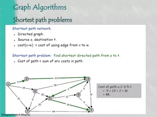
5. 4.9 4.3 1.8 B E G I 2.1 2.7 4.9 4.5 1.8 1.7 1.5 4.1 4.2 D H J 4.3 A 4.9 4.5 3.1 1.3 4.8 4.3 2.8 3.4 C F K 3.8 2.6 Shortest Path Tree …Costs are Random - Changing... Costs of the edges are determined on-the-fly Cost BE : 1.79 ; 1.68 ; 2.01, …..

6. The Static Algorithms • Dijkstra or Bellman-Ford’s solutions are unacceptably inefficient in dynamic environments. • Such static algorithms involve • Recomputing the shortest path tree “from scratch” • Done each time a topological change occurs.

7. Previous Dynamic Algorithms • Spira and Pan (1975): Very early work, proven theoretically to be inefficient. • McQuillan et al. (1980): Very early work, not proven at all. • Ramalingam and Reps (1996): Recent work, fully-dynamic solution. • Franciosa et al. (1997): Recent work, semi-dynamic solution. • Frigioni et al. (2000): Recent work, fully-dynamic solution.

8. Ramalingam and Reps’ Algorithm Edge-Insertion • Maintains a priority queue containing vertices • Priorities equal to their distance from the end-point of the inserted edge. • When a vertex having a minimum priority is extracted from the queue, all the outgoing edges are processed. Edge-Deletion • Phase I: Determines the vertices/edges affected by the deletion. • Phase II: Determines the new output value for all the affected vertices and updates the shortest path tree.

9. Frigioni et al.’s Algorithm Weight-Decrease • Based on “Output updates”. • No. of Output Updates = No. of vertices that change the distance from the source, on unit change in the graph. • If decreasing a weight changes the distance of the terminating end of the inserted vertex, a global priority queue is used to compute the new distances from the source. • Unlike the Ramalingam/Reps’ algorithm, on dequeuing a vertex, not all the edges leaving it are scanned.

10. Frigioni et al.’s Algorithm (Cont’d) Weight-Increase Based on the following node-coloring scheme: • Marking a node qwhite, which changes neither the distance from s nor the parent in the tree rooted in s • Marking a node qred, which increases the distance from s, • marking a node qpink, which preserves its distance from s, but replaces the old parent in the tree rooted in s.

11. Frigioni et al.’s Algorithm (Cont’d) Weight-Increase Three main phases: • Update local data-structures at the end-points of the affected edge, and check whether any distances change. • Color the vertices repeatedly by extracting vertices with minimum priority. • Compute the new distances for the red vertices.

12. Learning Automata • Previously used to model biological learning systems. • Can be used to find the optimal action. • How is learning accomplished?

13. {c1, ..., cr} Random Environment Learning Automaton Learning Automata … The Feedback Loop • Random Environment (RE) • Learning Automata (LA) • Set of actions {1, ..., r} • Reward/Penalty • Action Probability Vector • Action Probability Updating Scheme: The LRIscheme.  = {1, ..., r}  = {0, 1}

14. Variable Structure LA • Defined in terms of • Action Probability Updating Schemes • Action probability vector is : [p1(t), ..., pr(t)]T • pi(t) = Probability of choosing i at time ‘t’ • Implemented using random number generator • Flexibility: • Different actions at two consecutive time instants •  Action probabilityUpdated Various ways

15. Categories of VSSA • Classification based on the type of the probability space: • Continuous • Discrete • Classification based on the learning paradigm: • Reward-Penalty schemes • Reward-Inaction schemes • Inaction-Penalty schemes

16. Categories of VSSA • Ergodicscheme • Limiting Distribution: Independent of initial distribution •  Used if Environment is Non-stationary •  LA won’t get locked into any of the given actions.

17. Categories of VSSA • Absorbingscheme • Limiting Distribution: Dependent of initial distribution •  Used if Environment is Stationary •  LA finally gets Absorbed into its final action. • Example: Linear Reward-Inaction (LRI) scheme.

18. LRI Scheme p1(n) p2(n) p3(n) p4(n) 0.4 0.3 0.1 0.2 • If 2 chosen && rewarded. • p2 increased; • p1, p3, p4 decreased linearly. = p1(n+1) p2(n+1) p3(n+1) p4(n+1) 0.36 1-0.36-0.9-0.18 0.09 0.18 0.36 0.37 0.09 0.18 = = 0 1 0 0 p1() p2() p3() p4() If 2 is the best action:

19. Our Solution • Current state-of-the-art:No Solution to the DSSSP • When the edge-weights are dynamically and stochastically changing.

20. Our Solution • Our solution … • Uses the Theory of Learning Automata (LA). • Extends the current models by encapsulating the problem within the field of LA. • Finds a shortest path in realistically occurring stochastic environments. • Finds a shortest path for the “average” underlying graph, dictated by an “Oracle” (also called the Environment). • Finds the “statistical” shortest path tree, that will be stable regardless of continuously changing weights.

21. Our Solution Model … The Automata • Station a LA at every node in the graph. • At every instance, the LA chooses a suitable edge from all the outgoing edges at that node, by interacting with the environment. • The LA requests the Environment for the current random weight for the edge it chooses. • The system computes the current shortest path using RR/FMN. • LA determines whether the choice it made should be rewarded/penalized.

22. Our Solution Model … The Environment • Consists of the overall dynamically changing graph. • Multiple edge-weights that change stochastically and continuously. • Changes : Based on a distribution • Unknown to the LA, • Known to the Environment. • The Environment supplies a Reward/Penalty signal to the LA.

23. Our Solution Model … Reward/Penalty • Updated shortest path tree is computed • Based on the action the LA chooses, and • The edge-weight the Environment provides. • The LA compares the cost with the current “average” shortest paths. • The LA • Infers whether the choice should be rewarded/penalized. • Updatesthe action probabilities using the LRIscheme.

24. 0.5 0.5 0.6 0.4 0.4 0.6 4.9 4.3 1.8 B E G I 2.1 2.7 4.9 4.5 1.8 1.7 1.5 4.1 4.2 D H J 4.3 A 4.5 3.1 1.3 4.8 4.3 0.5 0.5 2.8 3.4 0.40 0.20 0.40 C F K 3.8 2.6 0.5 0.5 0.4 0.6 0.5 0.5 Shortest Path Tree …Updated Action Probability Vectors 4.9

25. INPUT • G(V,E) = A dynamically changing graph with simultaneous multiple stochastic edge updates occurring • iters = total number of iterations. • λ = learning parameter. • OUTPUT • A converged graph that has all the shortest path information. • Values of all action probability vectors. • ASSUMPTION • The algorithm maintains an action probability vector, P = {p1(n), p2(n) … pr(n)}, for each node of the graph. LASPA: The Proposed Algorithm

26. LASPA ALGORITHM 1 Obtaina snapshot of the directed graph with each edge having a random weight. This edge-weight is based on the random call for an edge. • Run Dijkstra’s Algorithm to determine the shortest path edges on the graph’s snapshot obtained in the first step. Based on this, update the action probability vector of each node - shortest path edges have an increased probability. • Randomly choose a node from the current graph. For that node, choose an edge based on the action probability vector. Request the edge-weight of this edge and recalculate the shortest path using either the RR or FMN algorithms. • Update the action probability vectors for all the nodes using the Reward-Inaction philosophy. • Repeat Steps 3-4 above until the algorithm has converged. LASPA: The Proposed Algorithm

27. Simulations … The Experiments • Experiment Set 1:Comparison of the performance of LASPA with FMN and RR for a fixed graph structure. • Experiment Set 2:Comparison of the performance results with variation in graph structures. • Experiment Set 3: Sensitivity of the performance of LASPA to the variation of certain parameters, while keeping others constant.

28. Simulations … The Performance Metrics • Average number of scanned edges per update operation. • Average number of processed nodes per update operation • Averagetime requiredper update operation.

29. Simulations … Experiment Set 1 Average Processed Nodes • Graph with 50 nodes, 20% sparsity. • Edge-weights with means between 1.0 and 5.0, and variances between 0.5 and 1.5 • Mixed sequences of 500 update operations.

30. Simulations … Experiment Set 1 (Cont’d) Average Time Per Update • Graph with 50 nodes, 20% sparsity. • Edge-weights with means between 1.0 and 5.0, and variances between 0.5 and 1.5 • Mixed sequences of 500 update operations.

31. Spar- sity FMN RR LASPA-FMN LASPA-RR 10% 4.0/0.0/110.0 5.94/10.0/550.0 3.12/0.0/770.0 3.66/0.0/110.0 30% 3.16/0.0/110.0 7.4/0.0/2310.0 2.9/0.0/390.0 3.36/0.0/110.0 50% 1.92/0.0/60.0 2.76/0.0/280.0 1.76/0.0/550.0 2.78/0.0/160.0 70% 2.64/0.0/330.0 2.02/0.0/220.0 2.04/0.0/110.0 2.5/0.0/60.0 90% 1.1/0.0/60.0 1.23/0.0/110.0 1.06/0.0/60.0 1.56/0.0/60.0 Simulations … Experiment Set 2 Variation in Graph Sparsity • Graphs with 100 nodes, varying sparsity. • Edge-weights with means between 1.0 and 5.0, and variances between 0.5 and 0.9, =0.9 • Mixed sequences of 500 update operations. • LASPA, on an average, performs better than RR/FMN. • Variation in the number of nodes show similar results. Table:Average/Min/Max Time Per Udate versus Sparsity

32. Simulations … Experiment Set 3 Sensitivity of results to the variation in Learning parameter. • Graph with 50 nodes, 20% sparsity. • Edge-weights with means between 1.0 and 5.0, and variances between 0.5 and 1.5 • Mixed sequences of 500 update operations. •  is varied. • Other metrics show similar results.

33. Conclusions • Novelty of our work • First reported LA solution to DSSSP. • Superior solution than the previous ones. • Existing algorithms can’t operate successfully in realistically occurring continuously changing stochastic environments. • Breakthrough solution that could have commercial value. • Practical usefulness of our algorithm • Telecommunications Networking • Transportation • Military • Future work • Evaluation on very large topologies. • Evaluation on real networks.