Download
1 / 22
220 likes | 302 Views
Some Comments on Model Performance for July 2002-June 2004. Dust ID Meeting November 10, 2005 Bishop, CA Ken Richmond Geomatrix. Presentation Outline. Comments on Air Sciences Model Performance Presentation RSIP “Lite” Model Performance

E N D
Some Comments on Model Performance for July 2002-June 2004 Dust ID Meeting November 10, 2005 Bishop, CA Ken Richmond Geomatrix
Presentation Outline • Comments on Air Sciences Model Performance Presentation • RSIP “Lite” Model Performance • 24-hour predictions using same techniques as in SCA simulations • Hourly predictions for the two episodes with the most SCAs • Area Source Resolution
Comments on Air Sciences Model Performance Presentation • Model Objectives • One of several lines of evidence for Supplemental Control Areas (SCAs)? • Area eroded before? • Visual observations • Within GPS boundary • Sand flux associated with high PM10 • Based on decision makers criteria • Where and when is good model performance more critical? • What measures can be used to evaluate the performance so decision makers can weigh the results against other evidence? • General Comments on Air Science Presentation • Poor performance is exaggerated while reasonable performance is not acknowledged • The exaggerated poor performance occurs during periods and concentration ranges that do not influence SCA selection • Why not the RSIP Performance Evaluation Procedures? • Selected on a collaborative basis after many months of discussion • Regulatory precedent
Comments on Air Sciences Model Performance Presentation • Should use 24-hr predictions and emphasize the conditions used to develop the SCAs • Use hourly measures to examine bias by condition, not paired in time performance • Performance goals based on Guidance for regional PM2.5 and O3 modeling are unrealistic • Ozone event concentrations vary by a factor of 10 from background to hourly peak or by a factor 2-3 across receptors affected • Owens Lake PM10 varies by 10,000 in an hour or within a few hundred meters • Data sampling/concentration ranges should be selected with care • Use of just TEOM (e.g. > 150 µg/m3) or just predictions to group data results in biased results. Grouping needs to be symmetric • Lower limit (especially for the TEOM) affects the geometric statistics. Geometric differences from 0.001 to 0.2, 0.1 to 20, 100 to 20,000 are the same • Select data from portions of the simulations that influence the SCAs. Grouping based on TEOM <150 µg/m3 have little relevance?
Mean Pred = 0.5 Mean Obs =.75
Mean Pred = 2/3 Mean Obs =2/3
Some Model Performance Results • Subset of the RSIP Model Performance Procedures • QQ-Plots, Log-Log Scatter Diagrams, simple statistics for P+O>150 µg/m3 • 24-hour Performance Examined for: • RSIP default K-factors • Revised 75% K-factors • Event specific K-factors when available (shown here) • SCAs were developed and contrasted for all 3 sets • Large Episode Model Performance • Most SCAs are identified during a couple of large events • Examples of episode performance for February 1-5, 2003 and March 29-April 2, 2004
R = .94 Rgeo =.54
R = .84 R_geo =.81 P+O>150 R = .81 R_geo = .66
R = .98 R_geo =.90 P+O>150 R = .97 R_geo = .80
R = .83 R_geo =.83 P+O>150 R = .80 R_geo = .74
R = .94 R_geo =.93 P+O>150 R = .92 R_geo = .95
Area Source Resolution • To Be Continued
Area Source Resolution • Pre-RSIP: ISCST3 Rectangles • Precise routine: initial plume corresponds to area source limits • Arbitrary orientations • Pre-RSIP CALPUFF: Volume Sources • Imprecise Gaussian shape • 250x250m Sources & Up • CALPUFF Rectangular Area Sources • Billed as an “ISCST3 like” precise routine • RSIP 1km x 1km, PUFF option • SCA analysis various sizes 250x250m & up corresponding to actual source boundaries, PUFF option • CALPUFF Area Source Imprecision • Only precise for SLUG option • Only precise for 1st time step • Upwind concentrations especially for aspect ratio >1 when winds are not aligned with area source