Download

1 / 23
230 likes | 241 Views
Whole Genome Sequencing, Comparative Genomics, & Systems Biology. Gene Myers University of California Berkeley. Cloning: BACs permit 100-250Kbp inserts Technology: Cycle sequencing (linear PCR) permits efficient sequencing of both insert ends

E N D
Whole Genome Sequencing, Comparative Genomics, & Systems Biology Gene Myers University of California Berkeley
Cloning: BACs permit 100-250Kbp inserts Technology: Cycle sequencing (linear PCR) permits efficient sequencing of both insert ends Capillaries improve accuracy & efficiency A History of Genome Sequencing • 1981: Sanger et al. sequence Lambda (50Kbp) by the shotgun method. • 1998: 3% of the human genome has been sequenced using a BAC-based hierachical plan. Common wisdom is that shotgun approach does not scale beyond BACs save for simple bacterial sequences.
Collect 6-10x sequence in a 5-5-1 ratio of three types of read pairs. Short Long 10Kbp 2Kbp Extra Long 50-150Kbp • Assemble into “scaffolds”, ordered runs of contigs with known spacing. Contig Gap (mean & std. dev. Known) Read pair (mates) + single highly automated process + only a handful of library constructions – assembly is much more difficult Whole Genome Shotgun Sequencing ~ 55million reads • Map scaffolds to genome with STS or other markers.
Identify and assembly all the unique genomic segments • Link together into scaffolds with paired reads • Back-fill interspersed repeats with “anchored reads” How to accomplish WGA in a nutshell
Evaluating WGA
Case Study: 3 Dros. Assemblies vs. Release 3 • Input: (Celera) 3.2M reads, 732K 2Kbp pairs, 548K 10Kbp pairs, (BDGP), 12K BAC pairs. • WGS1: Dec. 1999, reported in Science 2000. Repeat walking removed, Stones debugged, SNP handling • WGS2: March 2001, time of Human publication Error correction introduced, improvements in unitig classification • WGS3: July 2002, last run on melanogaster
WGS1 WGS2 WGS3 Rel. 3 99.91% # of Scaffolds Covering Rel. 3 55 63 53 13 98.93% Total Mb Spanned 116.39 117.44 117.6 116.91 Total Mb of Rel. 3 Spanned 116.4 116.5 116.8 -------- Total Mb of Sequence 114.15 115.83 116.42 116.87 Total Mb of Rel. 3 Sequence 114.1 115 115.6 -------- N50 Scaffold Length (in Mb) 10.85 14.45 13.89 18.5 Number of Gaps 2,173 2,315 1,130 44 Mean Contig Length (in kb) 52.2 49.5 102 2,335 Mean Gap Length (in bp) 1,531 912 1,335 --------- Coverage of Release 3 In addition 20.7Mbp of heterochromatic sequence was assembled (WGS3), containing 31 known proteins and 266 newly predicted genes. 58% of Rel. 3 gaps were interspersed repeat, 12% were tandem repeats (WGS3).
# segs # base pairs # segs # base pairs # segs # base pairs WGS1 WGS2 WGS3 2,125 113.30 Mb 2,270 Aligned Segments 114.41 Mb 1,087 114.99 Mb Local Errors 9 68.33 kb 7 9.80 kb 3 5.64 kb Repeat Errors 25 42.52 kb 1 0.66 kb 1 0.98 kb Gross misassemblies 3 10.69 kb 0 0 O&O Errors vs. Release 3
Errors / 10 kb WGS1 WGS2 WGS3 All Sequence 4.12 2.23 1.1 In Tandem Repeats 95.2 61.4 48.8 In Interspersed Repeats 78.2 15.8 9.62 In Unique Sequence 1.82 1.31 0.38 > 10 bp from gap 1.37 1.02 0.29 > 50 bp from gap 1.32 0.95 0.26 Sequencing Error Rates vs. Release 3
Solid State Sequencing in Pico-wells: • Operational next year • 25-50Mbp per instrument/day in 50bp reads, .3-1Kbp pairs (vs. 1-2Mbp per inst./day in 800bp, 2-10Kbp pairs) • Applications: Resequencing, BAC drafts at 99% • Detecting dNTP incoporations by fixed PolII complex: • Operational 5-10 years from now • 1-10Gbp per instrument/day in 100Kbp reads (they can be 30-50% noise)! • Assembly will not be difficult. • Nanopore • My opinion: not knowable, could be 50 years.
Comparative Gene Finding
Mouse is smaller than Human: ~15% expansion of euchromatin Syntenic Anchors Human (21) Sequence anchor: >50bp at >75% id. & bidirectionally unique Mouse (16) Mbp Mbp
Protein-level synteny Human chromosome 6 Mouse chromosome 17
Computational Gene Finding GENE: Stop Codon Acceptor Site Donor Site Start Codon GT AG ATG TRANSCRIPT: • Computational Gene finding: Identification of coordinates of coding regions. • ‘Clues’ that differentiate coding from non-coding regions. • Cellular machinery (ribosome,spliceosome) recognizes specific signals that mark gene boundaries.
Computational Gene Finding (Homology) • Comparative (Genewise, Procrustes, Sim4) • Perform well when homolog has strong similarity. Performance tapers off with decrease in sequence similarity. • Performance is (or, should be) independent of sequence composition. • Difficult to find good homologs.
Full Length cDNA’s: Alternate Splicing Courtesy Terry Gaasterland, Rockefeller
Gene Finding (Ab Initio Methods) • Gene structure is identified by the most likely parse of the sequence through an appropriate HMM (weighted finite automaton) (ex: Genscan, Genie…). • Fairly accurate, with well understood procedures for training models and parsing. • Recent results (multi-gene examples) indicates that further improvements are desirable (Guigo’99).
1D Methods: Summary • Homology: • Very specific and accurate • Can sample only abundunt genes and full-length is hard • Ab Initio: • Good sensitivity for presence (85%) but weak for exon (60%) and gene (10%), also very non-specific (20%). • Main drivers of recognition are: • Splice site • No stop codon in exon • Some bias in hexamer coding frequency • Mouse vs. Human Homology (50-100 million years): • 85% of exons in a TBlastX hit • 85% amino acid identity in a hit • 25% of TBlastX hits contain a true exon
2D: Homology (Sagot et al., Huson & Bafna) Require gene models (splice sites + start + no-stop) in both genomes that have high homology: Human Mouse Performance is better than 1D HMM with weak splice site model
Twinscan (Brent et al.): Target Evidence Mask (0/1) cDNA, other evidence SLAM (Pachter et al., Durbin et al.): Given training set of known genes and “correctly” alignments learn HMM over k 2D HMMs: Given training set of known genes and evidence mask learn HMM over {0/1}
Outcomes • Exon prediction (must get splice junctions right) • SN 63% 68% • SP 58% 66% • Gene prediction (must get every exon) • SN 15% 24% • SP 10% 14% • A lot of improvement possible ?