Relational Query Optimization
370 likes | 579 Views
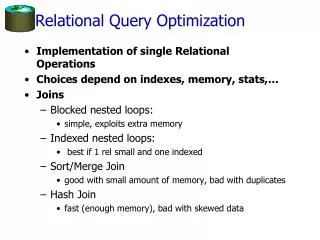
Relational Query Optimization. Overview of Query Optimization. Evaluation Plan : Tree of R.A. ops, with choice of alg for each op. Each operator typically implemented using a `pull’ interface: when an operator is `pulled’ for the next output tuples, it `pulls’ on its inputs and computes them.

Relational Query Optimization
E N D
Presentation Transcript
Overview of Query Optimization • Evaluation Plan:Tree of R.A. ops, with choice of alg for each op. • Each operator typically implemented using a `pull’ interface: when an operator is `pulled’ for the next output tuples, it `pulls’ on its inputs and computes them. • Two main issues: • For a given query, what plans are considered? • Algorithm to search plan space for cheapest (estimated) plan. • How is the cost of a plan estimated? • Ideally: Want to find best plan. • Practically: Avoid worst plans!
Evaluation of Expressions • So far: we have seen algorithms for individual operations • Alternatives for evaluating an entire expression (operator) tree • Materialization: generate results of an expression whose inputs are relations or are already computed, materialize (store) it on disk. Repeat. • Pipelining: pass on tuples to parent operations even as an operation is being executed
Materialization • Materialized evaluation: evaluate the expression bottom-up, storing intermediate results on disk • E.g., in figure below, compute and store • then compute the store its join with customer, and finally compute the projections on customer-name.
Materialization (Cont.) • Materialized evaluation is always applicable • Cost of writing results to disk and reading them back can be quite high • Overall cost = Sum of costs of individual operations + cost of writing intermediate results to disk • Double buffering: use two output buffers for each operation, when one is full write it to disk while the other is getting filled • Allows overlap of disk writes with computation and reduces execution time
Pipelining • Pipelined evaluation : evaluate several operations simultaneously, passing the results of one operation on to the next. • E.g., in previous expression tree, don’t store result of • instead, pass tuples directly to the join. Similarly, don’t store result of join, pass tuples directly to projection. • For pipelining to be effective, use evaluation algorithms that generate output tuples even as tuples are received for inputs to the operation. • Pipelines can be executed in two ways: demand driven and producer driven
Pipelining (Cont.) • In demand driven or lazyevaluation • Each operation is implemented as an iterator implementing the following operations • init() • E.g. file scan: initialize file scan, store pointer to beginning of file as state • next() • E.g. for file scan: Output next tuple, and advance and store file pointer • close()
Pipelining (Cont.) • In produce-driven or eager pipelining • Operators produce tuples eagerly and pass them up to their parents • Buffer maintained between operators, child puts tuples in buffer, parent removes tuples from buffer • if buffer is full, child waits till there is space in the buffer, and then generates more tuples • System schedules operations that have space in output buffer and can process more input tuples
Schema for Examples Sailors (sid: integer, sname: string, rating: integer, age: real) Reserves (sid: integer, bid: integer, day: dates, rname: string) • Similar to old schema (except rname) • Reserves: • Each tuple is 40 bytes long, 100 tuples per page, 1000 pages. • Sailors: • Each tuple is 50 bytes long, 80 tuples per page, 500 pages.
Query Blocks: Units of Optimization SELECT S.sname FROM Sailors S WHERE S.age IN (SELECT MAX (S2.age) FROM Sailors S2 GROUP BY S2.rating) • An SQL query is parsed into a collection of queryblocks, and these are optimized one block at a time. • Nested blocks are usually treated as calls to a subroutine, made once per outer tuple. (This is an over-simplification, but serves for now.) Outer block Nested block
Query Optimization • Query Rewriting: • Given a relational algebra expression produce and equivalent expression that can be evaluated more efficiently • Plan generator: • Choose the best algorithm for each operator given statistics about the database, main memory constraints and available indices
Transformation of Relational Expressions • Two RA expressions are equivalent if they produce the same results on the same inputs • In SQL, inputs and outputs are multisets of tuples • Two expressions in the multiset version of the relational algebra are said to be equivalent if on every legal database instance the two expressions generate the same multiset of tuples • An equivalence rule says that expressions of two forms are equivalent • Can replace expression of first form by second, or vice versa
Equivalence Rules 1. Conjunctive selection operations can be deconstructed into a sequence of individual selections. 2. Selection operations are commutative. 3. Only the last in a sequence of projection operations is needed, the others can be omitted. • Selections can be combined with Cartesian products and theta joins. • (R1 X R2) = R1 R2 • 1(R1 2 R2) = R11 2 R2
Equivalence Rules (Cont.) 5. Theta-join operations (and natural joins) are commutative.R1 R2 = R2 R1 6. (a) Natural join operations are associative: (R1 R2) R3 = R1 (R2 R3)(b) Theta joins are associative in the following manner:(R1 1 R2) 2 3R3 = R1 1 3 (R22 R3) where 2involves attributes from only R2 and R3.
Equivalence Rules (Cont.) • The selection operation distributes over the theta join operation under the following two conditions: (a) When all the attributes in 0 involve only the attributes of one of the expressions (R1) being joined.0R1 R2) = (0(R1)) R2 (b) When 1 involves only the attributes of R1 and2 involves only the attributes of R2. 1 R1 R2) = (1(R1)) ( (R2))
Equivalence Rules (Cont.) 8. The projections operation distributes over the theta join operation as follows: (a) if involves only attributes from L1 L2: (b) Consider a join E1 E2. • Let L1 and L2 be sets of attributes from E1 and E2, respectively. • Let L3 be attributes of E1 that are involved in join condition , but are not in L1 L2, and • let L4 be attributes of E2 that are involved in join condition , but are not in L1 L2.
Example with Multiple Transformations • Query: Find the names of all customers with an account at a Brooklyn branch whose account balance is over $1000. cname((branch-city = “Brooklyn” balance > 1000 (branch (account depositor))) • Transformation using join associatively (Rule 6a): cname((branch-city = “Brooklyn” balance > 1000 (branch account) depositor) Second form provides an opportunity to apply the “perform selections early” rule, resulting in the subexpression branch-city = “Brooklyn” (branch) balance > 1000 (account)
Enumeration of Alternative Plans • There are two main cases: • Single-relation plans • Multiple-relation plans • For queries over a single relation, queries consist of a combination of selects, projects, and aggregate ops: • Each available access path (file scan / index) is considered, and the one with the least estimated cost is chosen. • The different operations are essentially carried out together (e.g., if an index is used for a selection, projection is done for each retrieved tuple, and the resulting tuples are pipelined into the aggregate computation).
Cost Estimation • For each plan considered, must estimate cost: • Must estimate costof each operation in plan tree. • Depends on input cardinalities. • We’ve already discussed how to estimate the cost of operations (sequential scan, index scan, joins, etc.) • Must also estimate size of result for each operation in tree! • Use information about the input relations. • For selections and joins, assume independence of predicates.
Cost Estimates for Single-Relation Plans • Index I on primary key matches selection: • Cost is Height(I)+1 for a B+ tree, about 1.2 for hash index. • Clustered index I matching one or more selects: • (NPages(I)+NPages(R)) * product of RF’s of matching selects. • Non-clustered index I matching one or more selects: • (NPages(I)+NTuples(R)) * product of RF’s of matching selects. • Sequential scan of file: • NPages(R). • Note: We discussed more detailed cost estimation already
Join Ordering • For all relations r1, r2, and r3, (r1r2) r3 = r1 (r2r3 ) • If r2r3 is quite large and r1r2 is small, we choose (r1r2) r3 so that we compute and store a smaller temporary relation.
Enumeration of Equivalent Expressions • Query optimizers use equivalence rules to generate equivalent expressions • 1st Approach: Generate all equivalent expressions • But... Very expensive • 2nd Approach: Exploit common sub-expressions: • when E1 is generated from E2 by an equivalence rule, usually only the top level of the two are different, subtrees below are the same and can be shared • E.g. when applying join associatively • Time requirements are reduced by not generating all expressions
Cost-Based Optimization • Consider finding the best join-order for r1r2 . . . rn. • There are (2(n – 1))!/(n – 1)! different join orders for the expression above. With n = 7, the number is 665280, with n = 10, thenumber is greater than 176 billion! • No need to generate all the join orders. Using dynamic programming, the least-cost join order for any subset of {r1, r2, . . . rn} is computed only once and stored for future use.
Dynamic Programming in Optimization • To find best join tree for a set of n relations: • To find best plan for a set S of n relations, consider all possible plans of the form: S1 (S – S1) where S1 is any non-empty subset of S. • Recursively compute costs for joining subsets of S to find the cost of each plan. Choose the cheapest of the 2n– 1 alternatives.
Join Order Optimization Algorithm procedure findbestplan(S)if (bestplan[S].cost )return bestplan[S]// else bestplan[S] has not been computed earlier, compute it nowfor each non-empty subset S1 of S such that S1 SP1= findbestplan(S1) P2= findbestplan(S - S1) A = best algorithm for joining results of P1 and P2 cost = P1.cost + P2.cost + cost of Aif cost < bestplan[S].cost bestplan[S].cost = costbestplan[S].plan = “execute P1.plan; execute P2.plan; join results of P1 and P2 using A”returnbestplan[S]
D D C C D B A C B A B A Queries Over Multiple Relations • Fundamental decision in System R: only left-deep join treesare considered. • As the number of joins increases, the number of alternative plans grows rapidly; we need to restrict the search space. • Left-deep trees allow us to generate all fully pipelined plans. • Intermediate results not written to temporary files. • Not all left-deep trees are fully pipelined (e.g., SM join).
Left Deep Join Trees • In left-deep join trees, the right-hand-side input for each join is a relation, not the result of an intermediate join.
Cost of Optimization • With dynamic programming time complexity of optimization with bushy trees is O(3n). • Space complexity is O(2n) • If only left-deep trees are considered, time complexity of finding best join order is O(n 2n) • Space complexity remains at O(2n) • Cost-based optimization is expensive, but worthwhile for queries on large datasets (typical queries have small n, generally < 10)
Heuristic Optimization • Cost-based optimization is expensive, even with dynamic programming. • Systems may use heuristics to reduce the number of choices that must be made in a cost-based fashion. • Heuristic optimization transforms the query-tree by using a set of rules that typically (but not in all cases) improve execution performance: • Perform selection early (reduces the number of tuples) • Perform projection early (reduces the number of attributes) • Perform most restrictive selection and join operations before other similar operations. • Some systems use only heuristics, others combine heuristics with partial cost-based optimization.
Enumeration of Left-Deep Plans • Left-deep plans differ only in the order of relations, the access method for each relation, and the join method for each join. • Enumerated using N passes (if N relations joined): • Pass 1: Find best 1-relation plan for each relation. • Pass 2: Find best way to join result of each 1-relation plan (as outer) to another relation. (All 2-relation plans.) • Pass N: Find best way to join result of a (N-1)-relation plan (as outer) to the N’th relation. (All N-relation plans.) • For each subset of relations, retain only: • Cheapest plan overall, plus • Cheapest plan for each interesting order of the tuples.
Enumeration of Plans (Contd.) • ORDER BY, GROUP BY, aggregates etc. handled as a final step, using either an `interestingly ordered’ plan or an additional sorting operator. • An N-1 way plan is not combined with an additional relation unless there is a join condition between them, unless all predicates in WHERE have been used up. • i.e., avoid Cartesian products if possible.
Cost Estimation for Multirelation Plans SELECT attribute list FROM relation list WHERE term1 AND ... ANDtermk • Consider a query block: • Maximum # tuples in result is the product of the cardinalities of relations in the FROM clause. • Reduction factor (RF) associated with eachtermreflects the impact of the term in reducing result size. Resultcardinality = Max # tuples * product of all RF’s. • Multi-relation plans are built up by joining one new relation at a time. • Cost of join method, plus estimation of join cardinality gives us both cost estimate and result size estimate
sname sid=sid rating > 5 bid=100 Sailors Reserves Sailors: B+ tree on rating Hash on sid Reserves: B+ tree on bid Example • Pass1: • Sailors: B+ tree matches rating>5, and is probably cheapest. However, if this selection is expected to retrieve a lot of tuples, and index is unclustered, file scan may be cheaper. • Still, B+ tree plan kept (because tuples are in rating order). • Reserves: B+ tree on bid matches bid=100; cheapest. • Pass 2: • We consider each plan retained from Pass 1 as the outer, and consider how to join it with the (only) other relation. • e.g., Reserves as outer: Hash index can be used to get Sailors tuples • that satisfy sid = outer tuple’s sid value.
SELECT S.sname FROM Sailors S WHERE EXISTS (SELECT * FROM Reserves R WHERE R.bid=103 AND R.sid=S.sid) Nested Queries • Nested block is optimized independently, with the outer tuple considered as providing a selection condition. • Outer block is optimized with the cost of `calling’ nested block computation taken into account. • Implicit ordering of these blocks means that some good strategies are not considered. The non-nested version of the query is typically optimized better. Nested block to optimize: SELECT * FROM Reserves R WHERE R.bid=103 AND S.sid= outer value Equivalent non-nested query: SELECT S.sname FROM Sailors S, Reserves R WHERE S.sid=R.sid AND R.bid=103
Summary • Query optimization is an important task in a relational DBMS. • Must understand optimization in order to understand the performance impact of a given database design (relations, indexes) on a workload (set of queries). • Two parts to optimizing a query: • Consider a set of alternative plans. • Must prune search space; typically, left-deep plans only. • Must estimate cost of each plan that is considered. • Must estimate size of result and cost for each plan node. • Key issues: Statistics, indexes, operator implementations.
Summary (Contd.) • Single-relation queries: • All access paths considered, cheapest is chosen. • Issues: Selections that match index, whether index key has all needed fields and/or provides tuples in a desired order. • Multiple-relation queries: • All single-relation plans are first enumerated. • Selections/projections considered as early as possible. • Next, for each 1-relation plan, all ways of joining another relation (as inner) are considered. • Next, for each 2-relation plan that is `retained’, all ways of joining another relation (as inner) are considered, etc. • At each level, for each subset of relations, only best plan for each interesting order of tuples is `retained’.