Download
1 / 17
210 likes | 806 Views
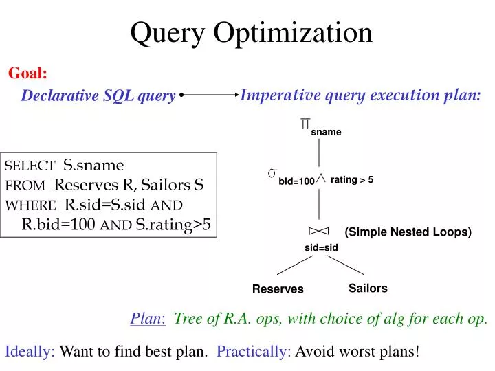
sname. rating > 5. bid=100 . (Simple Nested Loops). sid=sid. Sailors. Reserves. Query Optimization. Goal:. Declarative SQL query. Imperative query execution plan:. SELECT S.sname FROM Reserves R, Sailors S WHERE R.sid=S.sid AND R.bid=100 AND S.rating>5.

E N D
sname rating > 5 bid=100 (Simple Nested Loops) sid=sid Sailors Reserves Query Optimization Goal: Declarative SQL query Imperative query execution plan: SELECT S.sname FROM Reserves R, Sailors S WHERE R.sid=S.sid AND R.bid=100 AND S.rating>5 Plan:Tree of R.A. ops, with choice of alg for each op. Ideally: Want to find best plan. Practically: Avoid worst plans!
Query Optimization Issues • Query rewriting: • transformations from one SQL query to another one using semantic properties. • Selecting query execution plan: • done on single query blocks (I.e., S-P-J blocks) • main step: join enumeration • Cost estimation: • to compare between plans we need to estimate their cost using statistics on the database.
sname sid=sid (Scan; (Scan; write to write to rating > 5 bid=100 temp T2) temp T1) Reserves Sailors sname rating > 5 bid=100 sid=sid Sailors Reserves Query Rewriting: Predicate Pushdown The earlier we process selections, less tuples we need to manipulate higher up in the tree (but may cause us to loose an important ordering of the tuples.
Query Rewrites: Predicate Pushdown (more complicated) Select bid, Max(age) From Reserves R, Sailors S Where R.sid=S.sid GroupBy bid Having Max(age) > 40 Select bid, Max(age) From Reserves R, Sailors S Where R.sid=S.sid and S.age > 40 GroupBy bid Having Max(age) > 40 • Advantage: the size of the join will be smaller. • Requires transformation rules specific to the grouping/aggregation • operators. • Won’t work if we replace Max by Min.
Query Rewrite: Predicate Movearound Sailing wizz dates: when did the youngest of each sailor level rent boats? Select sid, date From V1, V2 Where V1.rating = V2.rating and V1.age = V2.age Create View V1 AS Select rating, Min(age) From Sailors S Where S.age < 20 GroupBy bid Create View V2 AS Select sid, rating, age, date From Sailors S, Reserves R Where R.sid=S.sid
Query Rewrite: Predicate Movearound Sailing wizz dates: when did the youngest of each sailor level rent boats? Select sid, date From V1, V2 Where V1.rating = V2.rating and V1.age = V2.age, age < 20 First, move predicates up the tree. Create View V1 AS Select rating, Min(age) From Sailors S Where S.age < 20 GroupBy bid Create View V2 AS Select sid, rating, age, date From Sailors S, Reserves R Where R.sid=S.sid
Query Rewrite: Predicate Movearound Sailing wizz dates: when did the youngest of each sailor level rent boats? Select sid, date From V1, V2 Where V1.rating = V2.rating and V1.age = V2.age, andage < 20 First, move predicates up the tree. Then, move them down. Create View V1 AS Select rating, Min(age) From Sailors S Where S.age < 20 GroupBy bid Create View V2 AS Select sid, rating, age, date From Sailors S, Reserves R Where R.sid=S.sid, and S.age < 20.
Query Rewrite Summary • The optimizer can use any semantically correct rule to transform one query to another. • Rules try to: • move constraints between blocks (because each will be optimized separately) • Unnest blocks • Especially important in decision support applications where queries are very complex.
Enumeration of Alternative Plans • Task: create a query execution plan for a single Select-project-join block (well, and aggregates). • Main principle: some sort of search through the set of plans. • Assume some cost estimation model; more later. • Single-relation block case (only select, project, aggregation): • Each available access path is considered, and the one with the least estimated cost is chosen. • The different operations are essentially carried out together (e.g., if an index is used for a selection, projection is done for each retrieved tuple, and the resulting tuples are pipelined into the aggregate computation).
D D C C D B A C B A B A Queries Over Multiple Relations • In principle, we need to consider all possible join orderings: • As the number of joins increases, the number of alternative plans grows rapidly; we need to restrict the search space. • System-R: consider only left-deep join trees. • Left-deep trees allow us to generate all fully pipelined plans:Intermediate results not written to temporary files. • Not all left-deep trees are fully pipelined (e.g., SM join).
Enumeration of Left-Deep Plans • Enumerated using N passes (if N relations joined): • Pass 1: Find best 1-relation plan for each relation. • Pass 2: Find best way to join result of each 1-relation plan (as outer) to another relation. (All 2-relation plans.) • Pass N: Find best way to join result of a (N-1)-relation plan (as outer) to the N’th relation. (All N-relation plans.) • For each subset of relations, retain only: • Cheapest plan overall, plus • Cheapest plan for each interesting order of the tuples.
Enumeration of Plans (Contd.) • ORDER BY, GROUP BY, aggregates etc. handled as a final step, using either an `interestingly ordered’ plan or an additional sorting operator. • An N-1 way plan is not combined with an additional relation unless there is a join condition between them, unless all predicates in WHERE have been used up. • i.e., avoid Cartesian products if possible. • In spite of pruning plan space, this approach is still exponential in the # of tables. • If we want to consider all (bushy) trees, we need only a slight modification to the algorithm.
Sailors: B+ tree on rating Hash on sid Reserves: B+ tree on bid sname sid=sid rating > 5 bid=100 Sailors Reserves Example • Pass 1: • Sailors: B+ tree matches rating>5, and is probably cheapest. However, if this selection is expected to retrieve a lot of tuples, and index is unclustered, file scan may be cheaper. • Still, B+ tree plan kept (tuples are in rating order). • Reserves: B+ tree on bid matches bid=100; cheapest. • Pass 2:We consider each plan retained from Pass 1 as the outer, and consider how to join it with the (only) other relation. • e.g., Reserves as outer: Hash index can be used to get Sailors tuples that satisfy sid = outer tuple’s sid value.
SELECT S.sname FROM Sailors S WHERE EXISTS (SELECT * FROM Reserves R WHERE R.bid=103 AND R.sid=S.sid) Nested Queries • Nested block is optimized independently, with the outer tuple considered as providing a selection condition. • Outer block is optimized with the cost of `calling’ nested block computation taken into account. • Implicit ordering of these blocks means that some good strategies are not considered. The non-nested version of the query is typically optimized better. Nested block to optimize: SELECT * FROM Reserves R WHERE R.bid=103 AND S.sid= outer value Equivalent non-nested query: SELECT S.sname FROM Sailors S, Reserves R WHERE S.sid=R.sid AND R.bid=103
Cost Estimation • For each plan considered, must estimate cost: • Must estimate costof each operation in plan tree. • Depends on input cardinalities. • Must estimate size of result for each operation in tree! • Use information about the input relations. • For selections and joins, assume independence of predicates. • We’ll discuss the System R cost estimation approach. • Very inexact, but works ok in practice. • More sophisticated techniques known now.
Statistics and Catalogs • Need information about the relations and indexes involved. Catalogstypically contain at least: • # tuples (NTuples) and # pages (NPages) for each relation. • # distinct key values (NKeys) and NPages for each index. • Index height, low/high key values (Low/High) for each tree index. • Catalogs updated periodically. • Updating whenever data changes is too expensive; lots of approximation anyway, so slight inconsistency ok. • More detailed information (e.g., histograms of the values in some field) are sometimes stored.
Size Estimation and Reduction Factors SELECT attribute list FROM relation list WHERE term1 AND ... ANDtermk • Consider a query block: • Maximum # tuples in result is the product of the cardinalities of relations in the FROM clause. • Reduction factor (RF) associated with eachtermreflects the impact of the term in reducing result size. Resultcardinality = Max # tuples * product of all RF’s. • Implicit assumption that terms are independent! • Term col=value has RF 1/NKeys(I), given index I on col • Term col1=col2 has RF 1/MAX(NKeys(I1), NKeys(I2)) • Term col>value has RF (High(I)-value)/(High(I)-Low(I))