Download

1 / 58
710 likes | 1.43k Views
Confounding in epidemiology. Maura Pugliatti, MD, PhD Associate Professor of Neurology Dept. of Clinical and Experimental Medicine, Unit of Clinical Neurology University of Sassari, Italy 1 st International Course of Neuroepidemiology Chisinau, Moldova, 24-28 Sept. 2012.

E N D
Confounding in epidemiology Maura Pugliatti, MD, PhDAssociate Professor of NeurologyDept. of Clinical and Experimental Medicine, Unit of Clinical NeurologyUniversity of Sassari, Italy 1st International Course of Neuroepidemiology Chisinau, Moldova, 24-28 Sept. 2012
“Confounding, the situation in which an apparent effect of an exposure on risk is explained by its association with other factors, is probably the most important cause of spurious associations in observational epidemiology” BMJ Editorial: “The scandal of poor epidemiological research” BMJ 2004;329:868-869 Definitions “Bias of the estimated effect of an exposure on an outcome, due to the presence of a common cause of the exposure and the outcome” Porta, 2008
Overview Causality: central concern of epidemiology Confounding: central concern when establishing causality Four approaches to understand confounding Avoiding and controlling for confounding is essential in health research
Causality Main application of epidemiology: to identify etiologic (causal) associations between exposure(s) and outcome(s) ? Exposure Outcome
Key biases in identifying causal effects: Causal Effect Random Error Confounding Information bias (misclassification) Selection bias Bias in inference Reporting & publication bias Bias in knowledge use RRcausal “truth” RRassociation Adapted from: Maclure, M, Schneeweis S. Epidemiology 2001;12:114-122.
Confounding: four approaches “Mixing of effects” Based on a priori criteria (classical approach) Data-based criteria “Counterfactual” and non-comparability approaches Overlapping
“Confounding is confusion, or mixing, of effects; the effect of the exposure is mixed together with the effect of another variable, leading to bias” Latin: “confundere” = “to mix together” Rothman KJ. Epidemiology. An introduction. Oxford: Oxford University Press, 2002
Association between birth order and Down Syndrome Data from Stark and Mantel (1966)
Association between maternal age and Down Syndrome Data from Stark and Mantel (1966)
Association between maternal age and Down Syndrome, stratified by birth order Data from Stark and Mantel (1966)
1. A confounder must be causally or non-causally associated with the exposure in the source population (study base) being studied; A factor is a confounder if 3 criteria are met: C E • 2. A confounder must be a causal risk factor (or a surrogate measure of a cause) for the disease in the unexposed cohort; and C D • 3. A confounder must not be an intermediate cause (not an intermediate step in the causal pathway between the exposure and the disease) X D E C
Exposure Disease (outcome) D E Intermediate cause Exposure Disease C E D Confounder C Szklo M, Nieto JF. Epidemiology: Beyond the basics. Aspen Publishers, Inc., 2000. Gordis L. Epidemiology. Philadelphia: WB Saunders, 4th Edition.
Confounder: ‘parent’ of the exposure not ‘daughter’ of the exposure!!! Exposure Disease E D Confounder C
Confounding factor: Maternal Age C Birth Order Down Syndrome D E
Simple causal graphs C E D Maternal age (C) can confound the association between multivitamin use (E) and the risk of certain birth defects (D) Hernan MA, et al. Causal knowledge as a prerequisite for confounding evaluation: an application to birth defects epidemiology. Am J Epidemiol 2002;155:176-84.
Complex causal graphs U C E D History of birth defects (C) may increase the chance of periconceptional vitamin intake (E). A genetic factor (U) could have been the cause of previous birth defects in the family, and could again cause birth defects in the current pregnancy (D) Hernan MA, et al. Causal knowledge as a prerequisite for confounding evaluation: an application to birth defects epidemiology. Am J Epidemiol 2002;155:176-84.
More complicated causal graphs Physical Activity Smoking A B BMI C U E D Bone fractures Calcium supplementation Source: Hertz-Picciotto
A factor is a confounder if: a) the effect measure is homogeneous across the strata defined by the confounder and b) the crude and common stratum-specific (adjusted) effect measures are unequal (“lack of collapsibility”) Usually evaluated using 2x2 tables, and simple stratified analyses to compare crude effects with adjusted effects “Collapsibility is equality of stratum-specific measures of effect with the crude (collapsed), unstratified measure” Porta, 2008, Dictionary
Crude vs. Adjusted Effects Crude: does not take into account the effect of the confounder Adjusted: accounts for the confounder Mantel-Haenszel method estimator Multivariate analyses (e.g. logistic regression) Confounding is likely when: RRcrude =/= RRadjusted ORcrude =/= ORadjusted
Stratified Analysis Crude 2 x 2 table Calculate Crude OR (or RR) Stratify by Confounder Calculate OR’s for each stratum If stratum-specific OR’s are similar, calculate adjusted OR (e.g. MH) Crude ORCrude Stratum 1 Stratum 2 OR1 OR2 If Crude OR = Adjusted OR, confounding is unlikely If Crude OR =/= Adjusted OR, confounding is likely
Ideal “causal contrast” between exposed and unexposed groups: “A causal contrast compares disease frequency under two exposure distributions, but in one target population during one etiologic time period” If the ideal causal contrast is met, the observed effect is the “causal effect” Maldonado & Greenland, Int J Epi 2002;31:422-29
Ideal counterfactual comparison to determine causal effects: Exposed cohort Iexp Initial conditions are identical in the exposed and unexposed groups, except for presence of exposure (=cause) Unexposed cohort Iunexp RRcausal = Iexp / Iunexp Maldonado & Greenland, Int J Epi 2002;31:422-29
What happens in reality? Exposed cohort Iexp Unexposed cohort Iunexp Substitute, unexposed cohort Isubstitute RRassoc = Iexp / Isubstitute
In this case: RRcausal = Iexp / Iunexp IDEAL RRassoc = Iexp / Isubstitute ACTUAL “Confounding is present if the substitute population represents imperfectly what the target would have been like under the counterfactual condition”
Simulating the counter-factual comparison:Experimental Studies: Randomized Clinical Trials Disease + Treated individuals Randomization Eligible population Disease - Disease + Untreated individuals Disease - compare rates Randomization helps to make the groups “comparable” (i.e. similar initial conditions) with respect to known and unknown confounders Confounding is unlikely at randomization - time t0
Disease + Exposed cohort Disease - Disease + Unexposed cohort Disease - Simulating the counter-factual comparison:Observational Studies: Cohort studies, case-control studies compare rates PRESENT FUTURE In observational studies, because exposures are not assigned randomly, attainment of exchangeability is impossible – “initial conditions” are likely to be different and the groups may not be comparable
Confounding:Observational studies vs randomized trials Example: Aspirin to reduce cardiovascular mortality
Confounding: adjustment and controls Control at the design stage Randomization Restriction Matching Control at the analysis stage Conventional approaches Stratified analyses Multivariate analyses Newer approaches Graphical approaches using DAGs Propensity scores Instrumental variables Marginal structural models
Options at the design stage: Randomization Reduces potential for confounding by generating groups that are fairly comparable with respect to known and unknown confounding variables Restriction Eliminates variation in the confounder (e.g. only recruiting one gender) Matching Involves selection of a comparison group that is forced to resemble the index group with respect to the distribution of one or more potential confounders
Randomization Randomization Only for intervention studies Definition: random assignment of study subjects to exposure categories To control/reduce the effect of confounding variables about which the investigator is unaware (i.e. both known and unknown confounders get distributed evenly because of randomization) Randomization does not always eliminate confounding Covariate imbalance in small trials “Maldistribution” of potentially confounding variables after randomization (“Table I: Baseline characteristics” in the randomized trial)
Randomization breaks any links between treatment and prognostic factors Confounder C Randomization X Exposure Disease (outcome) D E
Restriction The distribution of the potential confounding factors does not vary across exposure or disease categories An investigator may restrict study subjects to only those falling with specific level(s) of a confounding variable Advantages of restriction straightforward, convenient, inexpensive (but, reduces recruitment!) Disadvantages of restriction Limits number of eligible subjects Limits ability to generalize the study findings Residual confounding Impossible to evaluate the relationship of interest at different levels of the confounder
Matching Matching is commonly used in case-control studies Match on strong confounder Types: Pair (individual) matching Frequency matching The use of matching usually requires special analysis techniques (e.g. matched pair analyses and conditional logistic regression)
Matching Disadvantages of matching Finding appropriate control subjects: difficult and expensive and limit sample size Confounder used to match subjects cannot be evaluated with respect to the outcome/disease Matching does not control for confounders other than those used to match The use of matching makes the use of stratified analysis very difficult Matching is most often used in case-control studies (prohibitive in a large cohort study) In a case-control study, matching may even introduce confounding
Controlling Confounding:At the analysis stageConventional approaches
Confounding is one type of bias that can be adjusted in the analysis (unlike selection and information bias) Options at the analysis stage: Stratification Multivariate methods To control for confounding in the analyses, confounders must be measured in the study Confounding: control at the analysis stage
Stratification Produce groups within which the confounder does not vary Evaluate the exposure-disease association within each stratum of the confounder
Stratified Analysis Crude 2 x 2 table Calculate Crude OR (or RR) Stratify by Confounder Calculate OR’s for each stratum If stratum-specific OR’s are similar, calculate adjusted OR (e.g. MH) Crude ORCrude Stratum 1 Stratum 2 OR1 OR2 If Crude OR = Adjusted OR, confounding is unlikely If Crude OR =/= Adjusted OR, confounding is likely
Confounding “pulls” the observed association away from the true association It can either exaggerate/over-estimate the true association (positive confounding) Example ORcausal = 1.0 ORobserved = 3.0 or It can hide/under-estimate the true association (negative confounding) Example ORcausal = 3.0 ORobserved = 1.0 Direction of Confounding
Multivariate Analysis Stratified analysis works best only in the presence of 1 or 2 confounders If the number of potential confounders is large, multivariate analyses offer the only real solution Can handle large numbers of confounders (covariates) simultaneously Based on statistical regression “models” E.g. logistic regression, multiple linear regression Always done with statistical software packages
Residual confounding Confounding that can persist, even after adjustment Unmeasured confounding Some variables were actually not confounders Confounders were measured with error (eg., misclassification) Categories of the confounder improperly defined
Effect modification and interaction Maura Pugliatti, MD, PhDAssociate Professor of NeurologyDept. of Clinical and Experimental Medicine, Unit of Clinical NeurologyUniversity of Sassari, Italy 1st International Course of Neuroepidemiology Chisinau, Moldova, 24-28 Sept. 2012
Definition • Biological interaction • Effect modification (“effect-measure modification”) • Heterogeneity of effects • Subgroup effects • Statistical Interaction • Deviation from a specified model form (additive or multiplicative)
Biological interaction “the interdependent operation of two or more biological causes to produce, prevent or control an effect”[Porta, Dictionary, 2008]
Multicausality and interdependent effects • Disease processes tend to be multifactorial: “multicausality” • The “one-variable-at-a-time” perspective has several limitations • Confounding and effect modification: manifestations of multicausality Schoenbach, 2000
Effect modification and statistical interaction • Two definitions (related): • Based on homogeneity or heterogeneity of effects • Interaction occurs when the effect of a risk factor (X) on an outcome (Y) is not homogeneous in strata formed by a third variable (Z, effect modifier) • “Differences in the effect measure for one factor at different levels of another factor” [Porta, 2008] • This is often called “effect modification” • Based on the comparison between observed and expected joint effects of a risk factor and a third variable • Interaction occurs when the observed joint effects of the risk factor (X) and third variable (Z) differs from that expected on the basis of their independent effects • This is often called “statistical interaction” Szklo & Nieto, Epidemiology: Beyond the basics. 2007
Definition based on homogeneity or heterogeneity of effects Effect of exposure on the disease is modified depending on the value of a third variable: the “effect modifier” Effect modifier Exposure Disease