Download
1 / 16
160 likes | 301 Views
Agricultural Policy Changes and Regional Economies: A Computable General Equilibrium (CGE) Analysis for 6 EU Member-States Dr. Demetrios Psaltopoulos and Dr. Eudokia Balamou TERA Conference October 18 th -19 th, 2007, Ferrara. MOTIVATION FOR AGRICULTURAL POLICY SIMULATION.

E N D
Agricultural Policy Changes and Regional Economies: A Computable General Equilibrium (CGE) Analysis for 6 EU Member-States Dr. Demetrios Psaltopoulos and Dr. Eudokia Balamou TERA Conference October 18th -19th, 2007, Ferrara
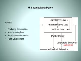
MOTIVATION FOR AGRICULTURAL POLICY SIMULATION • RECENT (FUNDAMENTAL) CAP REFORM Most subsidies replaced by SFP – Cross Compliance - Modulation • CAP REFORMS Have significantly influenced rural areas (farm + non-farm incomes; economic activity; distribution, etc.) – Some evidence of New-CAP impacts • IMPACT ASSESSMENT Several studies – rather ex-ante. Various predictions ranging from modest to ‘non-modest’. • PREDICTION DOMAINS Farm income change; rural economic activity; distribution of gains; structural adjustment (incl. farm size, orientation, specialization); farm labour costs, etc.
MOTIVATION FOR AGRICULTURAL POLICY SIMULATION TERA • Seeks to analyze the impacts of the role of agriculture and (especially) farm support • Assess (rural and urban) economic effects associated with changes in agricultural policy • TERA CGE MODELS Capture multi-product nature of agriculture – Structure allows simulations to portray economic interdependencies within each economy + rural/urban interactions
AGRICULTURE IN THE STUDY AREAS Seems rather important • Employment share: IT: 14-35%; SC:12.5%; FI: 8%; GR: 38%; LV: 47%; CZ: 6.6% • UAA: Very high share in total land (46 – 70%) – Mostly LFA • Structures: Mostly family farms (less in CZ) – Small size (mostly in Greece) – declining • Production: Specific to area-context(s) • Labour: Mostly family labour – large share of old-age (in some cases) – seasonal labour (in some cases)
DEFINITION OF AGRICULTURAL POLICY SCENARIOS • Rather “extreme” • AGPCUT Abolishment (100%) of all agric. subsidies • DECOUPLE Full (100%) Decoupling (govt. transfer to Agric. HHS) – New CAP SFP • PILLAR 2 100% reduction of agric. subsidies with transfer of all funds to Pillar 2 (investment demand for Construction) • MODULATION 20% of the SFP funds goes to Pillar 2 – Axis 3 (CAP Health-check?)
MODELLING AGRICULTURAL POLICY SCENARIOS Base Year of SAM Tables • Greece 2004 • Czech 2002 • Italy 2003 • Scotland 2003 • Finland 2002 • Latvia 2005
AGPCUT Scenario • Indirect Activity Tax Rate (Agricultural Sector) • Domestic Activity of the Agricultural Sector Domestic Production of Agricultural Products Agricultural Sector linked with other Sectors of the Economy Changes in Sectors Dom. Activ. Total Domestic Activity-Domestic Production Employment, GDP, Exports, Private Cons.
RESULTS % Changes from AGPCUT Scenario
DECOUPLE Scenario • Transfers to Agr. HHS Income of Agr. HHS and also affects other HHS income • Private Consumption Levels of Agr. HHS But what happens to other HHS Consumption? What happens to farm-linked sectoral activity? What Happens to Prices? Sectoral Domestic Activity-Domestic Production Employment, GDP
RESULTS % Changes from DECOUPLE Scenario
PILLAR 2/Modulation Scenarios • Exogenous Investment Demand of the Construction Commodity • Domestic Production of the Construction Commodity • Domestic Activity of the Construction Sector What Happens with the Domestic Activity of other Sectors? Usually positive effects in other sectors, but possible trade-off due to decrease in AgrHHS Consumption. Employment, GDP
RESULTS % Changes from PILLAR 2 Scenario
RESULTS % Changes from MODULATION Scenario
RESULTS Changes in Rents/ Prices In all countries and scenarios Agricultural Rents (very high in Scotland and Finland up to 67%) Consumer Price of Agricultural Products Consumer Prices of the Secondary (except Greece and Scotland in Agpcut) and Tertiary (except Decouple and Modulation in Scotland) Producer Prices of Agricultural Products • Producer Prices of Secondary (except Greece- Czech and Latvia under Pillar 2) Producer Prices of Tertiary (except Scotland in Decouple and Modulation and Latvia in Pillar 2)
CONCLUSIONS • Subsidies are important for the rural economies cutting them off results in losses but these do not seem drastic. • Cutting subsidies “hurts” others than just farmers agric. linked sectors seem to experience hard times if agricultural activity is not subsidized • Full Decoupling seems to cause higher negative effects compared to the elimination of subsidies (but Agr. HHS incomes rise) • Transfer of SFP funds to Pillar 2 measures rather “improves” the situation (except Agr. HHS income) • Impacts of Modulation Scenario: a bit worse than subsidies elimination, but better than Full Decoupling • Modulation scenario is better for Latvia
CONCLUSIONS • GDP GR, IT, FIN Rural GDP in all scenarios CZ Urban GDP in all scenarios except Agpcut UK Urban GDP LV Rural GDP in Agpcut and Modulation • Employment GR, CZ, IT, FIN, UK Rural Employment LV Rural in Agpcut and Modulation