Download
1 / 43
440 likes | 645 Views
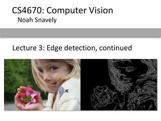
CS4670: Computer Vision. Noah Snavely. Lecture 2: Edge detection. From Sandlot Science. Announcements. Project 1 released, due Friday, September 7. Edge detection. Convert a 2D image into a set of curves Extracts salient features of the scene More compact than pixels.

E N D
CS4670: Computer Vision Noah Snavely Lecture 2: Edge detection From Sandlot Science
Announcements • Project 1 released, due Friday, September 7
Edge detection • Convert a 2D image into a set of curves • Extracts salient features of the scene • More compact than pixels TexPoint fonts used in EMF. Read the TexPoint manual before you delete this box.: AAA
Origin of Edges Edges are caused by a variety of factors surface normal discontinuity depth discontinuity surface color discontinuity illumination discontinuity
Images as functions… • Edges look like steep cliffs
intensity function(along horizontal scanline) first derivative edges correspond toextrema of derivative Characterizing edges • An edge is a place of rapid change in the image intensity function image Source: L. Lazebnik
Image derivatives • How can we differentiate a digital image F[x,y]? • Option 1: reconstruct a continuous image, f, then compute the derivative • Option 2: take discrete derivative (finite difference) How would you implement this as a linear filter? : : Source: S. Seitz
Image gradient • The gradient of an image: The gradient points in the direction of most rapid increase in intensity • The edge strength is given by the gradient magnitude: • The gradient direction is given by: • how does this relate to the direction of the edge? Source: Steve Seitz
Image gradient Source: L. Lazebnik
Effects of noise Noisy input image Where is the edge? Source: S. Seitz
h f * h Solution: smooth first f To find edges, look for peaks in Source: S. Seitz
f Associative property of convolution • Differentiation is convolution, and convolution is associative: • This saves us one operation: Source: S. Seitz
2D edge detection filters derivative of Gaussian (x) Gaussian
Derivative of Gaussian filter y-direction x-direction
The Sobel operator Common approximation of derivative of Gaussian • The standard defn. of the Sobel operator omits the 1/8 term • doesn’t make a difference for edge detection • the 1/8 term is needed to get the right gradient value
Sobel operator: example Source: Wikipedia
Example • original image (Lena)
Finding edges gradient magnitude
Finding edges where is the edge? thresholding
Non-maximum supression • Check if pixel is local maximum along gradient direction • requires interpolating pixels p and r
Finding edges thresholding
Finding edges thinning (non-maximum suppression)
Canny edge detector MATLAB: edge(image,‘canny’) • Filter image with derivative of Gaussian • Find magnitude and orientation of gradient • Non-maximum suppression • Linking and thresholding (hysteresis): • Define two thresholds: low and high • Use the high threshold to start edge curves and the low threshold to continue them Source: D. Lowe, L. Fei-Fei
Canny edge detector • Still one of the most widely used edge detectors in computer vision • Depends on several parameters: J. Canny, A Computational Approach To Edge Detection, IEEE Trans. Pattern Analysis and Machine Intelligence, 8:679-714, 1986. : width of the Gaussian blur high threshold low threshold
Canny edge detector original Canny with Canny with • The choice of depends on desired behavior • large detects “large-scale” edges • small detects fine edges Source: S. Seitz
first derivative peaks Scale space (Witkin 83) • Properties of scale space (w/ Gaussian smoothing) • edge position may shift with increasing scale () • two edges may merge with increasing scale • an edge may not split into two with increasing scale larger Gaussian filtered signal
Image Scissors • Today’s Readings • Intelligent Scissors, Mortensen et. al, SIGGRAPH 1995 Aging Helen Mirren
Extracting objects • How could this be done? • hard to do manually • hard to do automatically (“image segmentation”) • pretty easy to do semi-automatically
Intelligent Scissors • Approach answers basic question • Q: how to find a path from seed to mouse that follows object boundary as closely as possible? • A: define a path that stays as close as possible to edges
Intelligent Scissors • Basic Idea • Define edge score for each pixel • edge pixels have low cost • Find lowest cost path from seed to mouse mouse seed • Questions • How to define costs? • How to find the path?
Let’s look at this more closely • Treat the image as a graph q c p • Graph • node for every pixel p • link between every adjacent pair of pixels, p,q • cost c for each link • Note: each link has a cost • this is a little different than the figure before where each pixel had a cost
Defining the costs q s c p r Want to hug image edges: how to define cost of a link? • good (low-cost) links follow the intensity edge • want intensity to change rapidly to the link • c – |intensity of r – intensity of s|
Defining the costs q s • c can be computed using a cross-correlation filter • assume it is centered at p c p r
1 1 -1 -1 Defining the costs q s c p r w • c can be computed using a cross-correlation filter • assume it is centered at p • A couple more modifications • Scale the filter response by length of link c. Why? • Make c positive • Set c = (max-|filter response|*length) • where max = maximum |filter response|*length over all pixels in the image
0 9 4 5 3 1 3 3 2 Dijkstra’s shortest path algorithm link cost • Algorithm • init node costs to , set p = seed point, cost(p) = 0 • expand p as follows: • for each of p’s neighbors q that are not expanded • set cost(q) = min( cost(p) + cpq, cost(q) )
9 5 4 1 0 3 1 3 2 1 9 3 4 5 3 1 3 3 2 Dijkstra’s shortest path algorithm • Algorithm • init node costs to , set p = seed point, cost(p) = 0 • expand p as follows: • for each of p’s neighbors q that are not expanded • set cost(q) = min( cost(p) + cpq, cost(q) ) • if q’s cost changed, make q point back to p • put q on the ACTIVE list (if not already there)
9 4 1 0 5 3 3 2 3 9 1 5 4 1 3 3 3 2 Dijkstra’s shortest path algorithm 2 3 5 2 3 3 4 • Algorithm • init node costs to , set p = seed point, cost(p) = 0 • expand p as follows: • for each of p’s neighbors q that are not expanded • set cost(q) = min( cost(p) + cpq, cost(q) ) • if q’s cost changed, make q point back to p • put q on the ACTIVE list (if not already there) • set r = node with minimum cost on the ACTIVE list • repeat Step 2 for p = r
Dijkstra’s shortest path algorithm 9 4 1 3 4 6 3 2 1 0 3 3 3 5 5 4 1 3 3 3 2 2 3 5 2 3 3 4 • Algorithm • init node costs to , set p = seed point, cost(p) = 0 • expand p as follows: • for each of p’s neighbors q that are not expanded • set cost(q) = min( cost(p) + cpq, cost(q) ) • if q’s cost changed, make q point back to p • put q on the ACTIVE list (if not already there) • set r = node with minimum cost on the ACTIVE list • repeat Step 2 for p = r
Dijkstra’s shortest path algorithm • Properties • It computes the minimum cost path from the seed to every node in the graph. This set of minimum paths is represented as a tree • Running time, with N pixels: • O(N2) time if you use an active list • O(N log N) if you use an active priority queue (heap) • takes fraction of a second for a typical (640x480) image • Once this tree is computed once, we can extract the optimal path from any point to the seed in O(N) time. • it runs in real time as the mouse moves • What happens when the user specifies a new seed?
Example Result Peter Davis