Download
1 / 26
260 likes | 479 Views
CAP 5415: Computer Vision Fall 2008. Lecture 6: Edge Detection. Announcements. PS 2 is available Please read it by Thursday During Thursday lecture, I will be going over it in some detail Monday - Computer Vision Distinguished Lecturer series. Edge Detection.

E N D
CAP 5415: Computer Vision Fall 2008 Lecture 6: Edge Detection
Announcements • PS 2 is available • Please read it by Thursday • During Thursday lecture, I will be going over it in some detail • Monday - Computer Vision Distinguished Lecturer series
Edge Detection “Nonetheless, experience building vision systems suggests that very often, interesting things are happening in an image at an edge and it is worth knowing where the edges are.” – Forsyth and Ponce in “Computer Vision- A Modern Approach
Simplest Strategy • Calculate the magnitude of the image gradient • Compare against a threshold
Problems • We get thick edges • Redundant, especially if we going to be searching in places where edges are found
Solution • Identify the local maximums • Called “non-maximal suppression”
Basic Idea • The gradient will be perpendicular to the edge • Search along the gradient for the maximum point (From Slides by Forsyth)
Implementation • Quantize the gradient orientation to a fixed number of orientations • Search along those lines in a window around points above a threshold (From Course Notes by Shah)
Comparison Gradient Thresholding With non-maximal suppression
Avoiding Non-Maximal Suppression • Can we formulate the problem so we can eliminate non-maximal suppression? • Remember: we want to find the maxima and minima of the gradient • Look for places where 2nd derivative is zero • Called zero-crossings (you may not see the 2nd derivative actually be zero)
Finding Zero-Crossings • The second derivative is directional, but we can us the Laplacian which is rotationally invariant • The image is usually smoothed first to eliminate noise • Computing Laplacian after filtering with a Gaussian is equivalent to convolving with a Laplacian of a Gaussian
The Laplacian of Gaussian • Sometimes called a center-surround filter • Response is similar to the response of some neurons in the visual cortex
Implementation • Filter with Laplacian of Gaussian • Look for patterns like {+,0,-} or {+,-} • Also known as the Marr-Hildreth Edge Detector
Disadvantages • Behaves poorly at corners (From Slides by Forsyth)
Noise and Edge Detection • Noise is a bad thing for edge-detection • Usually assume that noise is white Gaussian noise (not likely in reality!) • Introduces many spurious edges • Low-pass filtering is a simple way of reducing the noise • For the Laplacian of Gaussian Method, it is integrated into the edge detection
Why does filtering with a Gaussian reduce noise? • Forsyth and Ponce’s explanation: “Secondly, pixels will have a greater tendency to look like neighbouring pixels — if we take stationary additive Gaussian noise, and smooth it, the pixel values of the resulting signal are no longer independent. In some sense, this is what smoothing was about — recall we introduced smoothing as a method to predict a pixel’s value from the values of its neighbours. However, if pixels tend to look like their neighbours, then derivatives must be smaller (because they measure the tendency of pixels to look different from their neighbours).” – from Computer Vision – A Modern Approach
How I like to see it • If F is the DFT of an image, then |F|2 is the power at each frequency • In the average power image, the power is equal at every frequency for i=1:10000 cimg=randn(128); cum=cum+abs(fft2(cimg)).^2; end
Remember: Energy in Images is concentrated in low-frequencies • When you low-pass filter, you’re retaining the relatively important low-frequencies and eliminating the noise in the high frequencies, where you don’t expect much image energy Log-Spectrum of the Einstein Image
Smoothing Fast • The Gaussian Filter is a separable filter • The 2D filter can be expressed as a series of 2 1D convolutions • For a 9x9 filter, a separable filter requires 18 computations versus 81 for the 2D filter = *
Further Improvements to the Gradient Edge-Dector • Fundamental Steps in Gradient-Based Edge Dection that we have talked about: • Smooth to reduce noise • Compute Gradients • Do Non-maximal suppression • There is one more heuristic that we can advantage of. • Edges tend to be continuous
Hysteresis Thresholding • Edges tend to be continuous • Still threshold the gradient • Use a lower threshold if a neighboring point is an edge • The “Canny Edge Detector” uses all of these heuristics
Martin, Fowlkes, and Malik gathered a set of human segmentations Is there better information than the gradient? From Martin, Fowlkes, and Malik (2004)
This is a precision-recall curve Texture and Color Help
The edge-detector was a classifier The type of classifier didn’t matter for this task Interesting Side-note
Next Time: • Fitting Lines to Edge Points • Binary Operations