Download

1 / 28
360 likes | 791 Views
Making practical progress in parameterizing turbulent mixing in the deep ocean. Sonya Legg Princeton University, NOAA-GFDL. The role of deep mixing in the general circulation. Cooling. Pole. Eq. convection. overflows. Overturning. Upwelling. tidal mixing.

E N D
Making practical progress in parameterizing turbulent mixing in the deep ocean Sonya Legg Princeton University, NOAA-GFDL
The role of deep mixing in the general circulation Cooling Pole Eq convection overflows Overturning Upwelling tidal mixing Diapycnal mixing is necessary to close the thermohaline circulation: tides and winds are the likely source of energy for deep diapycnal mixing. z Climate models need physically based parameterizations of spatially and temporally varying tidal mixing: here we will focus on tidal mixing.
Tidal Energy Budget Munk and Wunsch, 1998 Most tidal energy is dissipated in coastal oceans, but the small amount dissipated in deep ocean has large impact on climate. Different climate scenarios (e.g. raising/lowering sealevel) would have different dissipation patterns.
Mechanisms of tidal mixing in deep ocean • 1/3 of energy from ocean tides is dissipated in deep ocean. • Used for mixing stratified ocean interior. • Some mixing local to topography, e.g. mid-ocean ridges, seamounts • Some energy carried throughout ocean by waves, leading to distributed mixing. Barotropic tides Rough topography Internal tides Local mixing Wave-topography interactions Wave-wave interactions Wave steepening and breaking • Unknowns • How much energy is extracted from tides? • How is it initially partitioned between waves and mixing? • Where do waves eventually break and cause mixing? Remote and local mixing Tidal energy flow chart. Global climate models do not simulate any part of this chain of events, not just the final mixing.
Where does tidal mixing happen? Observations (Polzin et al, 1997) show interior mixing is concentrated over rough topography, e.g. mid-ocean ridges and seamounts
Evidence for tidal mixing over a knife-edged ridge: the Hawaiian Ocean Mixing Experiment (Klymak et al, 2005) Diffusivity (estimated from measured dissipation) enhanced over ridge Dissipation scales with M2 tidal energy flux (Klymak et al, 2005)
Governing parameters for tidal flow over topography Topography: height h, width L, depth H Flow: speed U, oscillation frequencyw H Others: coriolis f, buoyancy frequency N Nondimensional parameters h Wave slope L Relative steepness Relative height Topography Tidal excursion Froude numbers Flow Analytical studies assume some or all of topographic/flow parameters are small – numerical simulations don’t have this restriction.
Internal tide generation by finite-amplitude barotropic tide The relevant question for mixing parameterization purposes: how much energy is extracted from the barotropic tide? • Early theoretical predictions (e.g. Bell 1974) assume gentle, low amplitude topography (g, h/H << 1). • Recent numerical simulations (e.g. Khatiwala, 2003) and theory (e.g. St Laurent et al, 2003) examine how tidal conversion depends on finite steepness g and relative height h/H, for small amplitude flow. • As energy conversion doubles in deep fluid. • As h/H 1, energy conversion is further increased. Khatiwala 2003 St Laurent et al, 2003 Knife-edge topography Gaussian topography Increasing g Increasing h/H Q: What happens when RL> 1, and Fr = U/(Nh) < 1?
Numerical simulations of finite amplitude tidal flow over Gaussian topography. • Key questions for parameterization development: • Do theoretical predictions hold for large amplitude flows? • How much of converted energy is dissipated locally v. radiated away? Low, wide, shallow topo Low, narrow, steep topo Tall, steep topo Baroclinic velocity snapshots from simulations of tidal flow over Gaussian topo with forcing amplitude U0=2cm/s (Legg and Huijts, 2006; using MITgcm). Steep topography leads to generation of internal tide beams: energy concentrated on wave characteristics.
Quantitative results: energy conversion Rate of energy conversion from barotropic tide Ratio of dissipation rate to conversion rate St Laurent et al prediction for steep topo, h/H=0.5 Bell’s prediction St Laurent et al prediction for steep topo, deep fluid Low, wide topography; low, narrow topography; tall wide topography; tall narrow topography Theoretical predictions of energy conversion agree well with numerical model results. For wider topo, only 10% of energy extracted from tide is dissipated locally; for narrow topo, much greater fraction. All from Legg and Huijts, 2006; using MITgcm
Probable cause of higher relative dissipation for narrowest topography: smaller vertical lengthscales in internal tide Low wide shallow topo Low narrow steep topo Narrowest topo is the only case without energy peak at lowest vertical mode. Tall steep topo Tall steep narrow topo (Legg and Huijts, 2006)
Observations of dependence of dissipation on topographic lengthscale Mid Atlantic ridge has much less total internal tide energy flux than Hawaii, but similar levels at high mode numbers (m>10). Dissipation levels, especially at depth, are similar, suggesting dissipation is a function of energy in high modes. St Laurent and Nash, 2004.
Are narrow beams the only location for dissipation/mixing? Low narrow steep topo Tall steep topo Dissipation is all in narrow beams, no hydraulic effects Possible transient internal hydraulic jumps are a location for overturning Isopycnal deflection by large amplitude tides: U0 = 24cm/s Large amplitude forcing over large amplitude steep topo leads to local overturns in internal hydraulic jump-like features. (Legg and Huijts, 2006) Q: Can internal hydraulic jumps be important at more moderate (i.e. realistic) forcing velocities?
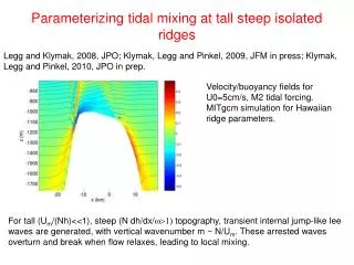
Example of internal hydraulic jumps with realistic forcing, topography: Hawaiian ridge Buoyancy field for U0=5cm/s, M2 tidal forcing. Hawaiian ridge is tall and steep. Hydraulic jumps develop over steep slope during downslope flow: at flow reversal, jumps propagate upslope as internal bores. -700m Asymmetric response: slope curvature is important. -1760m 46km Stratification and topography data from Kaena ridge courtesy of Jody Klymak and HOME researchers (Legg, 2006)
Transient hydraulics We would expect an internal wave to be unable to propagate against the flow if Group velocity is proportional to vertical wavelength So we might expect the flow to be supercritical to internal tides of wavelength lz< lc. For Hawaiian ridge parameters, lc = 465m at U0=5cm/s, so we expect transient hydraulic control of features below this scale. To have a hydraulic jump, flow must transition from supercritical to subcritical as it flows downslope, i.e. depth change within tidal period must be significant. where Depth change is significant if i.e. So transient hydraulic jumps may be possible if slope is sufficiently steep
Hawaiian ridge: Dependence of overturning on slope dh/dx(max) = 0.2, smooth dh/dx(max) = 0.2 Real topography dh/dx(max) = 0.1 dh/dx(max) = 0.06 Snapshots of U(color) and buoyancy (contours) just after flow reversal, all with U0=5cm/s Borelike features are found only for dh/dx(max) >> s, combined with a region of dh/dx = s at the top of the slope (Legg, 2006)
Dependence of overturning on flow amplitude U0=2cm/s U0=5cm/s U0=10cm/s Snapshots of U (color) and buoyancy (contours) just after flow reversal, for dh/dx(max) = 0.2. Larger amplitude flow increases extent and vigor of overturning.
Influence of internal bores on dissipation Log10 dissipation (time-averaged) for U0=5cm/s, dh/dx=0.2 Time-averaged dissipation for all simulations at location of maximum dissipation (h=-1170m) The region affected by internal bores has an order of magnitude higher dissipation than the internal wave beams. Steep slopes and large amplitude flows have largest dissipation.
Possible explanation of ``flow-reversal’’ mixing events (Aucan et al,2006) observed at mooring on Hawaiian ridge flank Potential temp dissipation currents Flow-reversal mixing event Downslope flow mixing event
Summary of progress on internal tide generation and local mixing • Recent theoretical advances in predicting energy conversion are supported by numerical simulations. • Only 10% of this energy is dissipated locally for most topographies • For very narrow topography dissipation is greatly enhanced and occurs mostly in internal tide beams. • Transient hydraulic jumps can produce a local enhancement of dissipation and mixing, when steep slopes are combined with large amplitude flows, especially when combined with breaking at critical slopes. Most of the baroclinic energy is in the form of radiating internal tides: Q: What is their fate?
Fate of internal tides: 1. Wave-wave interactions: (a) Parametric Subharmonic Instability MacKinnon and Winters, 2006 At latitudes where 2f < w(M2), PSI transfers energy into subharmonic with larger wavenumbers. When 2f = w(M2) (at 28.9 degrees) dissipation is greatly enhanced.
Fate of internal tides: 1. Wave-wave interactions: (b) steady-state continuum Garret-Munk-like spectrum is steady state result of wave-wave interactions (Caillol and Zeitlin, DAO, 2000) E(w,k) ~ w-2m-2 for w >> f Site D spectra (Garrett and Munk) (taken from Lvov et al, 2005)
Fate of internal tides: 2. Reflection from critical slopes: generation of internal bores Wave breaking is induced by reflection from near-critical slope, i.e. when . Buoyancy field for 1st mode internal tide Numerical simulations demonstrate mixing is possible at all shapes of critical slopes, provided 200m 3km Legg and Adcroft, 2003. so that reflected wave Fr > 1.
Fate of internal tides: 3. Scattering from corrugated slope With corrugations, high mode structure seen in velocity profiles Source: scattering of internal tide generated at shelf-break Scenario: internal tide generated at shelf break, with tidal forcing U=10cm/s reflecting from continental slope: possible description of TWIST region (Nash et al, 2004) Without corrugations With corrugations Cross-slope velocities at t=3.14 M2 periods Cross-slope velocity profiles at x=60km (Legg, 2004)
Tidal energy flow chart revisited…. Barotropic tides Simulations show that only 10% of energy is dissipated locally, except for very narrow topography. Rough topography 90% 10% Internal tides Local mixing Dissipation is located in beams and at near-critical slopes. Wave-topography interactions Wave-wave interactions Simulations have shown where internal tides will break and cause mixing – on slopes near critical angle. For slopes within a range of critical angle PSI Wave steepening and breaking Remote and local mixing
Parameterizing tidal mixing in ocean models St Laurent et al, 2002, implemented in GFDL MOM by Simmons et al, 2004 Spatially variable diffusivity: Where: q = fraction of energy dissipated locally – set to 1/3. This should be a function of the horizontal length-scales of the topography. G = mixing efficiency – set to 0.2 (this could be refined if DNS suggests it is necessary) K0= constant background diffusivity, accounting for remote mixing: Need to account for spatial variations in remote mixing, e.g. internal tide breaking, PSI at critical latitude. E(x,y) = energy extracted from barotropic tide: F(z) = vertical structure function: z = vertical decay scale – set to 500m. Does not account for preferred locations of mixing: e.g. beams, critical slopes.
Example of current tidal mixing parameterization Parameterized diffusivity due to tidal mixing in S. Atlantic (St Laurent et al, 2002)
Conclusions • Energetically consistent parameterizations of tidal mixing are now becoming a possibility. These parameterizations must include estimates of: • Energy conversion from the barotropic tide; • 2. The fraction of this energy used for local mixing and the spatial distribution of this mixing; • 3. The internal wave field generated by the tides; • 4. The locations of internal wave breaking, and the mixing thus generated. Many questions still remain, and theoretical, observational and numerical work are all needed to answer them. But we mustn’t be afraid to use what we already know, however approximate, to improve climate models!