Download
1 / 54
550 likes | 691 Views
Gas furnace data, cont. How should the sample cross correlations between the prewhitened series be interpreted?. pwgas<-prewhiten(gasrate,CO2,ylab="CCF") print(pwgas ) $ccf Autocorrelations of series ‘X’, by lag

E N D
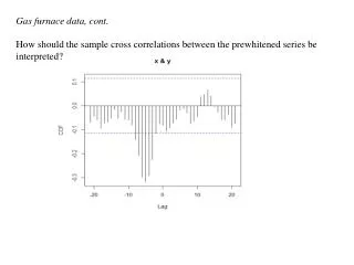
Gas furnace data, cont. How should the sample cross correlations between the prewhitened series be interpreted?
pwgas<-prewhiten(gasrate,CO2,ylab="CCF") print(pwgas) $ccf Autocorrelations of series ‘X’, by lag -21 -20 -19 -18 -17 -16 -15 -14 -13 -12 -11 -10 -9 -8 -7 -6 -5 -4 -3 -0.069 -0.044 -0.060 -0.092 -0.073 -0.069 -0.053 -0.015 -0.054 -0.026 -0.059 -0.060 -0.081 -0.141 -0.208 -0.299 -0.318 -0.292 -0.226 -2 -1 0 1 2 3 4 5 6 7 8 9 10 11 12 13 14 15 16 -0.116 -0.077 -0.083 -0.108 -0.093 -0.073 -0.058 -0.018 -0.013 -0.030 -0.077 -0.065 -0.045 0.039 0.047 0.067 0.041 -0.004 -0.026 17 18 19 20 21 -0.058 -0.060 -0.038 -0.091 -0.075 $model Call: ar.ols(x = x) Coefficients: 1 2 1.0467 -0.2131 Intercept: -0.2545 (2.253) Order selected 2 sigma^2 estimated as 1492
k = –3 What does this say about
Since the first significant spike occurs at k = –3 it is natural to set b = 3 • Rules-of-thumb: • The order of the numerator polynomial, i.e. s is decided upon how many significant spikes there are after the first signifikant spike and before the spikes start to die down. s =2 • The order of the denominator polynomial, i.e. r is decided upon how the spikes are dying down. • exponential : choose r = 1 • damped sine wave: choose r = 2 • cuts of after lag b + s : choose r = 0 • r = 1
Using the arimax command we can now try to fit this model without specifying any ARMA-structure in the full model and then fit an ARMA to the residuals. Alternatively we can expand to get an infinite terms expression in which we cut the terms corresponding with lags after the last lag with a significant spike in the sample CCF.
The last significant spike is for k = –8 Hence, we can use OLS (lm) to fit the temporary model and then model the residuals with a proper ARMA-model
model1_temp2 <- lm(CO2[1:288]~gasrate[4:291]+gasrate[5:292]+gasrate[6:293]+gasrate[7:294]+gasrate[8:295]+gasrate[9:296]) summary(model1_temp2) Call: lm(formula = CO2[1:288] ~ gasrate[4:291] + gasrate[5:292] + gasrate[6:293] + gasrate[7:294] + gasrate[8:295] + gasrate[9:296]) Residuals: Min 1Q Median 3Q Max -7.1044 -2.1646 -0.0916 2.2088 6.9429 Coefficients: Estimate Std. Error t value Pr(>|t|) (Intercept) 53.3279 0.1780 299.544 < 2e-16 *** gasrate[4:291] -2.7983 0.9428 -2.968 0.00325 ** gasrate[5:292] 3.2472 2.0462 1.587 0.11365 gasrate[6:293] -0.8936 2.3434 -0.381 0.70325 gasrate[7:294] -0.3074 2.3424 -0.131 0.89570 gasrate[8:295] -0.6443 2.0453 -0.315 0.75300 gasrate[9:296] 0.3574 0.9427 0.379 0.70491 --- Signif. codes: 0 ‘***’ 0.001 ‘**’ 0.01 ‘*’ 0.05 ‘.’ 0.1 ‘ ’ 1 Residual standard error: 3.014 on 281 degrees of freedom Multiple R-squared: 0.1105, Adjusted R-squared: 0.09155 F-statistic: 5.82 on 6 and 281 DF, p-value: 9.824e-06
acf(rstudent(model1_temp2)) pacf(rstudent(model1_temp2)) AR(2) or AR(3), probably AR(2)
model1_gasfurnace <- arima(CO2[1:288],order=c(2,0,0),xreg=data.frame(gasrate_3=gasrate[4:291],gasrate_4=gasrate[5:292],gasrate_5=gasrate[6:293],gasrate_6=gasrate[7:294],gasrate_7=gasrate[8:295], gasrate_8=gasrate[9:296])) print(model1_gasfurnace) Call: arimax(x = CO2[1:288], order = c(2, 0, 0), xreg = data.frame(gasrate_3 = gasrate[4:291], gasrate_4 = gasrate[5:292], gasrate_5 = gasrate[6:293], gasrate_6 = gasrate[7:294], gasrate_7 = gasrate[8:295], gasrate_8 = gasrate[9:296])) Coefficients: ar1 ar2 intercept gasrate_3 gasrate_4 gasrate_5 gasrate_6 gasrate_7 gasrate_8 1.8314 -0.8977 53.3845 -0.3382 -0.2347 -0.1517 -0.3673 -0.2474 -0.3395 s.e. 0.0259 0.0263 0.3257 0.1151 0.1145 0.1111 0.1109 0.1139 0.1119 sigma^2 estimated as 0.1341: log likelihood = -122.35, aic = 262.71 Note! With use only of xreg we can stick to the command arima
tsdiag(model1_gasfurnace) Some autocorrelation left in residuals
Forecasting a lead of two time-points (Works since the CO2 is modelled to depend on gasrate lagged 3 time-points) predict(model1_gasfurnace,n.ahead=2,newxreg=data.frame(gasrate[2:3],gasrate[3:4],gasrate[4:5],gasrate[5:6],gasrate[6:7],gasrate[7:8])) $pred Time Series: Start = 289 End = 290 Frequency = 1 [1] 56.76652 57.52682 $se Time Series: Start = 289 End = 290 Frequency = 1 [1] 0.3662500 0.7642258
Modelling Heteroscedasticity Exponential increase, but it can also be seen that the variance is not constant with time. A log transformation gives a clearer picture
Normally we would take first-order differences of this series to remove the trend (first-order non-stationarity)
The variance seems to increase with time, but we can rather see clusters of values with constant variance. For financial data, this feature is known as volatility clustering.
Correlation pattern? Not indicating non-stationarity. A clearly significant correlation at lag 19, though.
Autocorrelation of the series of absolute changes Clearly non-stationary!
If two variables X and Y are normally distributed Corr(X,Y) = 0 X and Y are independent Corr(|X|,|Y|) = 0 If the distributions are not normal, this equivalence does not hold In a time series where data are non-normally distributed The same type of reasoning can be applied to squared values of the time series. Hence, a time series where the autocorrelations are zero may still possess higher-order dependencies.
Another example : Stationary? Just noise spikes?
Ljung-Box tests for spurious data No evidence for any significant autocorrelations! LB_plot <- function(x,K1,K2,fitdf=0) { output <- matrix(0,K2-K1+1,2) for (i in 1:(K2-K1+1)) { output[i,1]<-K1-1+i output[i,2]<-Box.test(x,K1-1+i,type="Ljung-Box",fitdf)$p.value } win.graph(width=4.875,height=3,pointsize=8) plot(y=output[,2],x=output[,1],pch=1,ylim=c(0,1),xlab="Lag",ylab="P-value") abline(h=0.05,lty="dashed",col="red")
Autocorrelations for squared values A clearly significant spike at lag 1
McLeod-LI’s test Ljung-Box’ test applied to the squared values of a series McLeod.Li.test(y=spurdata) All P-values are below 0.05!
qqnorm(spurdata) qqline(spurdata) Slight deviation from the normal distribution Explains why there are linear dependencies between squared values, although not between original values
Jarque-Bera test A normal distribution is symmetric Moreover, the distribution tails are such that The sample functions sample skewness sample kurtosis can therefore be used as indicators of whether the sample comes from a normal distribution or not (they should both be close to zero for normally distributed data).
The Jarque-Bera test statistic is defined as and follows approximately a 2-distribution with two degrees of freedom if the data comes from a normal distribution. Moreover, each term is approximately 2-distributed with one degree of freedom under normality. Hence, if data either is too skewed or too heavily or lightly tailed compared with normally distributed data, the test statistic will exceed the expected range of a 2-distribution .
With R skewness can be calculated with the command skewness(x, na.rm = FALSE) and kurtosis with the command kurtosis(x, na.rm = FALSE) (Both come with the package TSA.) Hence, for the spurious time series we compute the Jarque-Bera test statistic and its P-value as JB1<-NROW(spurdata)*((skewness(spurdata))^2/6+ (kurtosis(spurdata))^2/24) print(JB1) [1] 31.05734 1-pchisq(JB1,2) [1] 1.802956e-07 Hence, there is significant evidence that data is not normally distributed
For the changes in log(General Index) we have the QQ plot In excess of the normal distribution JB2< NROW(difflogIndex)*((skewness(difflogIndex))^2/6+ (kurtosis(difflogIndex))^2/24) print(JB2) [1] 313.4869 1-pchisq(JB2,2) [1] 0 P-value so low that it is represented by 0!
ARCH-models ARCH stands for Auto-Regressive Conditional Heteroscedasticity The conditional variance or conditional volatility given the previous values of the time series. The ARCH model of order q [ARCH(q)] is defined as where {t } is white noise with zero mean and unit variance (a special case of et ) Engle R.F, Winner of Nobel Memorial Prize in Economic Sciences 2003 (together with C. Granger)
Modelling ARCH in practice Consider the ARCH(1).model
Now, let {t} will be white noise [not straightforward to prove, but Yt is constructed so it will have zero mean. Hence the difference between Yt2 and E(Yt2 | Y1, … , Yt –1 ) (which is t) can intuitively be realized must be something with zero mean and no correlation with values at other time-points] This extends by similar argumentation to ARCH(q)-models, i.e. the squared values Yt2 should satisfy an AR(q)
Application to “spurious data” example If an AR(q) model should be satisfied, the order can be 1 or two (depending on whether the interpretation of the SPAC renders one or two significant spikes.
Try AR(1) spur_model<-arima(spurdata^2,order=c(1,0,0)) print(spur_model) Call: arima(x = spurdata^2, order = c(1, 0, 0)) Coefficients: ar1 intercept 0.4410 0.3430 s.e. 0.0448 0.0501 sigma^2 estimated as 0.3153: log likelihood = -336.82, aic = 677.63
tsdiag(spur_model) Satisfactory?
Thus, the estimated ARCH-model is Prediction of future conditional volatility:
GARCH-models For purposes of better predictions of future volatility more of the historical data should be allowed to be involved in the prediction formula. The Generalized Auto-Regressive Conditional Heteroscedastic model of orders p and q [ GARCH(p,q) ] is defined as i.e. the current conditional volatility is explained by previous squared values of the time series as well as previous conditional volatilities.
For estimation purposes, we again substitute Hence, Yt2 follows an ARMA(max(p,q), p )-model
Note! An ARCH(q)-model is a GARCH(0,q)-model A GARCH(p,q)-model can be shown to be weakly stationary if A prediction formula can be derived as a recursion formula, now including conditional volatilities several steps backwards. See Cryer & Chan, page 297 for details.
Example GBP/EUR weekly average exchange rates 2007-2012 (Source: www.oanda.com) Non-stationary in mean (to slow decay of spikes)
First-order differences Apparent volatility clustering. Seems to be stationary in mean, though
Correlation pattern of squared values? Difficult to judge upon
EACF table AR/MA 0 1 2 3 4 5 6 7 8 9 10 11 12 13 0 x x x x x x x x x o o x o o 1 x o o x o o o o o o o o o o 2 x x o x o o o o o o o o o o 3 x x x x o o o o o o o o o o 4 x x o o x o x o o o o o o o 5 x x x o o o o o o o o o o o 6 x x o o o o x o o o o o o o 7 o o x o o o x o o o o o o o ARMA(1,1) ARMA(2,2) Candidate GARCH models: ARMA(1,1) 1 = max(p,q) GARCH(0,1) [=ARCH(1)] or GARCH(1,1) ARMA(2,2) 2 = max(p,q) GARCH(0,2, GARCH(1,2) or GARCH(2,2) Try GARCH(1,2) !
model1<-garch(diffgbpeur,order=c(1,2)) ***** ESTIMATION WITH ANALYTICAL GRADIENT ***** I INITIAL X(I) D(I) 1 1.229711e-04 1.000e+00 2 5.000000e-02 1.000e+00 3 5.000000e-02 1.000e+00 4 5.000000e-02 1.000e+00 IT NF F RELDF PRELDF RELDX STPPAR D*STEP NPRELDF 0 1 -1.018e+03 1 7 -1.019e+03 8.87e-04 1.15e-03 1.0e-04 1.2e+10 1.0e-05 6.73e+06 2 8 -1.019e+03 2.13e-04 2.95e-04 1.0e-04 2.0e+00 1.0e-05 5.90e+00 3 9 -1.019e+03 2.34e-05 3.00e-05 7.0e-05 2.0e+00 1.0e-05 5.69e+00 4 17 -1.025e+03 5.32e-03 9.66e-03 4.0e-01 2.0e+00 9.2e-02 5.68e+00 5 18 -1.025e+03 6.78e-04 1.61e-03 2.2e-01 2.0e+00 9.2e-02 7.59e-02 6 19 -1.026e+03 8.91e-04 1.80e-03 5.0e-01 1.9e+00 1.8e-01 5.02e-02 7 21 -1.030e+03 3.30e-03 2.14e-03 2.5e-01 1.8e+00 1.8e-01 7.51e-02 8 23 -1.030e+03 5.68e-04 5.78e-04 3.9e-02 2.0e+00 3.7e-02 1.87e+01 9 25 -1.030e+03 6.15e-05 6.64e-05 3.7e-03 2.0e+00 3.7e-03 1.00e+00 10 28 -1.031e+03 2.15e-04 2.00e-04 1.5e-02 2.0e+00 1.5e-02 1.11e+00 11 30 -1.031e+03 4.32e-05 4.02e-05 2.9e-03 2.0e+00 2.9e-03 8.17e+01 12 32 -1.031e+03 8.65e-06 8.04e-06 5.7e-04 2.0e+00 5.9e-04 4.13e+03 13 34 -1.031e+03 1.73e-05 1.61e-05 1.1e-03 2.0e+00 1.2e-03 3.89e+04 14 36 -1.031e+03 3.46e-05 3.22e-05 2.3e-03 2.0e+00 2.3e-03 8.97e+05 15 38 -1.031e+03 6.96e-06 6.43e-06 4.5e-04 2.0e+00 4.7e-04 1.29e+04 16 41 -1.031e+03 2.23e-07 1.30e-07 9.0e-06 2.0e+00 9.4e-06 8.06e+03 17 43 -1.031e+03 2.04e-08 2.57e-08 1.8e-06 2.0e+00 1.9e-06 8.06e+03 18 45 -1.031e+03 6.24e-08 5.15e-08 3.6e-06 2.0e+00 3.8e-06 8.06e+03 19 47 -1.031e+03 1.03e-07 1.03e-07 7.2e-06 2.0e+00 7.5e-06 8.06e+03 20 49 -1.031e+03 2.93e-08 2.06e-08 1.4e-06 2.0e+00 1.5e-06 8.06e+03 21 59 -1.031e+03 -4.30e-14 1.70e-16 6.5e-15 2.0e+00 8.9e-15 -1.37e-02 ***** FALSE CONVERGENCE ***** FUNCTION -1.030780e+03 RELDX 6.502e-15 FUNC. EVALS 59 GRAD. EVALS 21 PRELDF 1.700e-16 NPRELDF -1.369e-02 I FINAL X(I) D(I) G(I) 1 3.457568e-05 1.000e+00 -1.052e+01 2 2.214434e-01 1.000e+00 -6.039e+00 3 3.443267e-07 1.000e+00 -5.349e+00 4 5.037035e-01 1.000e+00 -1.461e+01
summary(model1) Call: garch(x = diffgbpeur, order = c(1, 2)) Model: GARCH(1,2) Residuals: Min 1Q Median 3Q Max -3.0405 -0.6766 -0.0592 0.6610 2.5436 Coefficient(s): Estimate Std. Error t value Pr(>|t|) a0 3.458e-05 1.469e-05 2.353 0.01861 * a1 2.214e-01 8.992e-02 2.463 0.01379 * a2 3.443e-07 1.072e-01 0.000 1.00000 b1 5.037e-01 1.607e-01 3.135 0.00172 ** --- Signif. codes: 0 ‘***’ 0.001 ‘**’ 0.01 ‘*’ 0.05 ‘.’ 0.1 ‘ ’ 1
Diagnostic Tests: Jarque Bera Test data: Residuals X-squared = 1.1885, df = 2, p-value = 0.552 Box-Ljung test data: Squared.Residuals X-squared = 0.1431, df = 1, p-value = 0.7052 Not every parameter significant, but diagnostic tests are OK. However, the problem with convergence should make us suspicious!
Try GARCH(0.2), i.e. ARCH(2) model11<-garch(diffgbpeur,order=c(0,2)) ***** ESTIMATION WITH ANALYTICAL GRADIENT ***** I INITIAL X(I) D(I) 1 1.302047e-04 1.000e+00 2 5.000000e-02 1.000e+00 3 5.000000e-02 1.000e+00 IT NF F RELDF PRELDF RELDX STPPAR D*STEP NPRELDF 0 1 -1.018e+03 1 7 -1.019e+03 8.27e-04 1.07e-03 1.0e-04 1.1e+10 1.0e-05 5.83e+06 2 8 -1.019e+03 2.25e-04 3.01e-04 1.0e-04 2.1e+00 1.0e-05 5.80e+00 3 9 -1.019e+03 1.37e-05 1.58e-05 7.0e-05 2.0e+00 1.0e-05 5.61e+00 4 17 -1.024e+03 5.37e-03 9.58e-03 4.0e-01 2.0e+00 9.2e-02 5.59e+00 5 18 -1.025e+03 2.04e-04 1.47e-03 2.4e-01 2.0e+00 9.2e-02 6.28e-02 6 28 -1.025e+03 4.45e-06 8.10e-06 2.6e-06 5.7e+00 9.9e-07 1.36e-02 7 37 -1.025e+03 4.75e-04 8.77e-04 1.1e-01 1.8e+00 4.8e-02 9.43e-03 8 38 -1.026e+03 1.03e-03 7.23e-04 1.3e-01 6.1e-02 4.8e-02 7.24e-04 9 39 -1.027e+03 5.04e-04 4.04e-04 9.8e-02 3.0e-02 4.8e-02 4.04e-04 10 40 -1.027e+03 8.14e-05 6.74e-05 4.0e-02 0.0e+00 2.3e-02 6.74e-05 11 41 -1.027e+03 5.52e-06 5.00e-06 1.1e-02 0.0e+00 7.0e-03 5.00e-06 12 42 -1.027e+03 1.30e-07 1.12e-07 1.4e-03 0.0e+00 7.8e-04 1.12e-07 13 43 -1.027e+03 2.19e-08 1.56e-08 5.2e-04 0.0e+00 3.5e-04 1.56e-08 14 44 -1.027e+03 7.58e-09 6.98e-09 6.2e-04 3.0e-02 3.5e-04 6.98e-09 15 45 -1.027e+03 2.30e-10 2.11e-10 1.1e-04 0.0e+00 5.8e-05 2.11e-10 16 46 -1.027e+03 3.88e-12 3.72e-12 8.2e-06 0.0e+00 5.8e-06 3.72e-12 ***** RELATIVE FUNCTION CONVERGENCE ***** FUNCTION -1.026796e+03 RELDX 8.165e-06 FUNC. EVALS 46 GRAD. EVALS 17 PRELDF 3.722e-12 NPRELDF 3.722e-12 I FINAL X(I) D(I) G(I) 1 8.171538e-05 1.000e+00 1.048e-01 2 2.631538e-01 1.000e+00 -3.790e-06 3 1.466673e-01 1.000e+00 8.242e-05
summary(model11) Call: garch(x = diffgbpeur, order = c(0, 2)) Model: GARCH(0,2) Residuals: Min 1Q Median 3Q Max -3.25564 -0.66044 -0.05575 0.63832 2.81831 Coefficient(s): Estimate Std. Error t value Pr(>|t|) a0 8.172e-05 1.029e-05 7.938 2e-15 *** a1 2.632e-01 9.499e-02 2.770 0.00560 ** a2 1.467e-01 5.041e-02 2.910 0.00362 ** --- Signif. codes: 0 ‘***’ 0.001 ‘**’ 0.01 ‘*’ 0.05 ‘.’ 0.1 ‘ ’ 1 All parameters are significant!
Diagnostic Tests: Jarque Bera Test data: Residuals X-squared = 3.484, df = 2, p-value = 0.1752 Box-Ljung test data: Squared.Residuals X-squared = 0.0966, df = 1, p-value = 0.7559 Diagnostic tests OK! In summary, we have the model Coefficient(s): Estimate Std. Error a0 8.172e-05 1.029e-05 a1 2.632e-01 9.499e-02 a2 1.467e-01 5.041e-02
Extension: Firstly, model the conditional mean, i.e. apply an ARMA-model to the first order differences ( an ARIMA(p,1,q) to original data) An MA(1) to the first-order differences seems appropriate cm_model<-arima(gbpeur,order=c(0,1,1)) Coefficients: ma1 0.4974 s.e. 0.0535 sigma^2 estimated as 0.0001174: log likelihood = 804.36, aic = -1606.72
tsdiag(cm_model) Seems to be in order
Now, investigate the correlation pattern of the squared residuals from the model