Download
1 / 76
790 likes | 963 Views
Biostat 209 Survival Data l. John Kornak April 2, 2013 John.kornak@ucsf.edu Reading VGSM 3.5 (review) and 6.1 - 6.2.4 http://www. epibiostat.ucsf.edu/biostat/vgsm/. Logistics. Lectures in 6702 every Tuesday ***EXCEPT*** additional lecture Thursday 4/19

E N D
Biostat 209Survival Data l • John Kornak • April 2, 2013 • John.kornak@ucsf.edu • Reading VGSM 3.5 (review) and 6.1 - 6.2.4 • http://www. • epibiostat.ucsf.edu/biostat/vgsm/
Logistics • Lectures in 6702 every Tuesday ***EXCEPT*** additional lecture Thursday 4/19 • 3 lectures survival analysis, 2 common biostatistical problems (Dr. Bacchetti), 3 repeated measures analysis (Dr. McCulloch) • Lectures are to be recorded and posted online • Note that homework given out by Dr. Bacchetti on 4/23 will be due at start of lecture on 4/25 • Grades based on 5 hw assignments (70%) + data analysis project (30%, due 5/18/12) • Check materials online and Biostat 209 discussion forum
Data Analysis Project • You need to complete a data analysis project • DOES NOT need to be on survival analysis, but would preferably use regression methods from Biostat 208 or 209 (see project guidelines on web site syllabus page) • A 2,000 word write-up is due on 5/23 • Presentation sessions on 5/28, 5/30, 6/4, or 6/6 • Email me by 4/9 (next Tuesday) • one brief paragraph description of your data, primary aim, possible/probable analysis plan • if working with a biostatistician? (name if yes) • if unavailable for any presentation sessions?
Data Analysis Project I will assign you to a faculty advisor Your advisor will meet with you (at your request) to help guide your analysis Students in groups of 6 for each presentation session (along with their advisors) 25 minute presentation, 3 hour session Your advisor will preside over your session
Survival Analysis Overview • Kaplan-Meir survival curves, logrank test • Cox proportional hazards modeling • Cox proportional hazard model checking • Extensions to the Cox proportional hazards model – time-varying covariates and overview of other methods competing risks, clustered data, interval censoring… • All methods illustrated with STATA
Survival data and censoring Functions for describing survival Kaplan-Meier (KM) curves Log-rank test Hazard function Proportional hazards model Cox model The Cox model in STATA (STCOX) In this lecture…
Survival data examples Years to death post surgery Weeks to relapse post rehab Minutes to infection post exposure Days to full recovery post surgery Different types of outcome with different effective time-scales
Example – Lymphoma data Survival (in days) of patients with lymphoma 6, 19, 32, 42, 42, 43*, 94, 126, 169*, 207, 211*, 227, 253, 255*, 270*, 310*, 316*, 335*, 346* … so what makes survival data special?
Example – Lymphoma data Survival (in days) of patients with lymphoma 6, 19, 32, 42, 42, 43*, 94, 126, 169*, 207, 211*, 227, 253, 255*, 270*, 310*, 316*, 335*, 346* … so what makes survival data special? Answer: * = still alive at end of follow up
Right Censoring Definition: A survival time is “right censored at time t” if we only know know that it is greater than t Example: A subject is followed for 18 months. Follow up ends and the subject is alive. The subject is then right censored at 18 months
(1) End of study Right censoring– not everyone is followed to death (2) (3) time • Subject followed to death (not censored) • Subject right censored by loss to follow up • Administratively censored: end of study Assume censoring is independent of treatment (non-informative, independent censoring)
Pediatric Kidney Transplant Example of Survival Data • United Network for Organ Sharing (UNOS) database • 9750 children under 18 yrs with kidney tx,1990-2002 • Outcome: time to death post transplant • 38,000 patient years, 429 deaths • What are predictors of post tx mortality? e.g., donor source: cadaveric v. living
Features of UNOS Data • Risk of death depends on length of follow-up (an individual has more chance of dying during the study if followed for 10 vs. 5 yrs) • Follow-up ranges from 1 day to 12.5 yrs • Most children are alive at end of study 438 of 9750 subjects have events (4.5%) • Thus, 95.5% of subjects are right censored
) ( UNOS Data
Survival Data in STATA • Declare the data to be survival data • Use stset command • stset Y, failure(δ) UNOS data: stset time, failure(indic) • In STATA, code δ carefully 1 should be event, 0 a censored observation read stset output summary to check
How can we analyze survival data? What happens if we try regression methods from Biostat 208?
Treat as Continuous? Question: What is the mean survival time? • Outcome: Time to Death • Problem:
Treat as Continuous? Outcome: Time to Death Problem: Most subjects still alive at study end Average time of death can be highly misleading Example: 100 subjects censored at 500 months and only 2 deaths at 1 and 3 months Average death time: 2 months....misleading! Question: What is the mean survival time? Mean time to death is not generally a useful summary for survival data!
Treat as Binary Proportion of subjects “alive” Question: what proportion of subjects survive?
Treat as Binary Proportion of subjects “alive” Different follow up times Requires an arbitrary cut-off time (e.g., 1 yr) What if a subject is censored at 360 days? their data is wasted: not followed for a year Deaths after 1 year are ignored, but most deaths may occur after 1 year! Question: what proportion of subjects survive?
Treat as Binary e.g., cut-off at 6 months or 1 year? observed censored Right and left censoring with no mechanism to deal with it!
Aims of a Survival Analysis • Summarize the distribution of survival times Tool: Kaplan-Meier estimates (of survival distribution) • Compare survival distributions between groups Tool: logrank test • Investigate predictors of survival Tool: Cox regression model Kaplan-Meier and logrank covered previously but will review
Functions for Describing Survival Probability density (distribution) - of death 0 t birth middle age old age
Functions for Describing Survival Survival function: the probability an individual will survive longer than a particular timet Pr(T>t ) S(t ) 1 Survival function often estimated by Kaplan-Meier (KM) estimator t 0 birth middle old
Estimating the Survival function with the Kaplan-Meier (KM) estimator The probability of death in any particular time interval can be estimated by: # observed deaths # at risk E.g. in a study of 2000 genetically bred mice, 230 died of heart failure between 0 and 3 weeks; estimate probability of death between 0 and 3 weeks to be 230/2000
Kaplan-Meier The survival curve is high at the start (because everyone is alive early on) and then the KM approach assumes that at the times we observe deaths in our dataset the survival curve should drop. To generate a KM estimated survival curve we consider intervals of “zero” length in time: Pr(death at time t ) = # observed deaths at time t # at risk at time t This leads to an instant drop in the survival curve of size “Pr(death at time t )” every time there is a death.
Kaplan-Meier Note that the “number at risk” in the denominator accounts for the censored data! Once a subject is censored they are no longer in the “at risk” group. The subsequent heights of drops for each death in the KM survival curve increases with each individual lost to follow up.
Kaplan-Meier Lymphoma data load lymph.dta // Stata commands stset Days, failure(relapse) sts list sts graph, censored(single) xtitle(Days) Beg. Net Survivor Days Total Fail Lost Function ------------------------------------------ 6 19 1 0 0.9474 19 18 1 0 0.8947 32 17 1 0 0.8421 42 16 2 0 0.7368 43 14 0 1 0.7368 94 13 1 0 0.6802 126 12 1 0 0.6235 169 11 0 1 0.6235 207 10 1 0 0.5611 211 9 0 1 0.5611 227 8 1 0 0.4910 253 7 1 0 0.4209 255 6 0 1 0.4209 270 5 0 1 0.4209 310 4 0 1 0.4209 316 3 0 1 0.4209 335 2 0 1 0.4209 346 1 0 1 0.4209 ------------------------------------------
Kaplan-Meier Lymphoma data load lymph.dta // Stata commands stset Days, failure(relapse) sts list sts graph, censored(single) xtitle(Days) Beg. Net Survivor Days Total Fail Lost Function ------------------------------------------ 6 19 1 0 0.9474 19 18 1 0 0.8947 32 17 1 0 0.8421 42 16 2 0 0.7368 43 14 0 1 0.7368 94 13 1 0 0.6802 126 12 1 0 0.6235 169 11 0 1 0.6235 207 10 1 0 0.5611 211 9 0 1 0.5611 227 8 1 0 0.4910 253 7 1 0 0.4209 255 6 0 1 0.4209 270 5 0 1 0.4209 310 4 0 1 0.4209 316 3 0 1 0.4209 335 2 0 1 0.4209 346 1 0 1 0.4209 ------------------------------------------ Median Survival time
Example – ALL Data 6-mercaptopurine (6-MP) maintenance thpy for children in remission from acute lymphoblastic leukemia (ALL) => outcome = time to relapse (weeks) Placebo: 1,1,2,2,3,4,4,5,5,8,8,8,8,11,11,12, 12,15,17,22,23 6-MP: 6,6,6,6*,7,9*,10,10*,11*,13,16,17*,19*,20*,22,23,25*,32*,34*,35* … Is there a difference in time to relapse of children on 6-MP vs. Placebo?
Curves for ALL data K-M Survival function Cumulative relapse incidence use leuk.dta, stset time, f(cens) sts graph, by(group) use leuk.dta, stset time, f(cens) sts graph, by(group) failure
Curves for ALL data K-M Survival function Cumulative relapse incidence use leuk.dta, stset time, f(cens) sts graph, by(group) use leuk.dta, stset time, f(cens) sts graph, by(group) failure Group Median Survival times
Logrank test for comparing Two Survival Curves • Logrank test compares different KM estimated survival functions (e.g. between groups) • Does not give estimated size of effect – use Kaplan-Meier curve (e.g. median survival times) or Cox Model for that purpose • The idea of the test is that (under the null hypothesis of “no group difference”) the proportion of deaths within each group at any time should not be too different than for the combined data from all groups: “All groups have the same survival distribution”.
Logrank test for comparing Two Survival Curves • Basically a large sample chi-square test: “observed – expected” across all time points • Main alternate test is the Wilcoxon test for censored data: used if either a) strong non-proportional hazards (see later), or b) want to give more weight to earlier events (weighted chi-square by number of observations in time interval) • Logrank test is recommended as a default
Logrank test for ALL data use leuk.dta stset time, f(cens) sts test group failure _d: cens analysis time _t: time Log-rank test for equality of survivor functions | Events Events group | observed expected --------+------------------------- 6 MP | 9 19.25 Placebo | 21 10.75 --------+------------------------- Total | 30 30.00 chi2(1) = 16.79 Pr>chi2 = 0.0000
Wilcoxon test for ALL data use leuk.dta stset time, f(cens) sts test group, wilcoxon failure _d: cens analysis time _t: time Wilcoxon (Breslow) test for equality of survivor functions | Events Events Sum of group | observed expected ranks --------+-------------------------------------- 6 MP | 9 19.25 -271 Placebo | 21 10.75 271 --------+-------------------------------------- Total | 30 30.00 0 chi2(1) = 13.46 Pr>chi2 = 0.0002
Summary of KM and logrank in STATA • stset command declares outcome as survival doesn’t need to be specified again • sts list, by(txtype)print Kaplan-Meier by variable txtype • sts graph, by(txtype) graph Kaplan-Meier by variable txtype • sts test txtype calculates logrank test for variable txtype
Aims of a Survival Analysis Summarize the distribution of survival times Tool: Kaplan-Meier estimates (of survival distribution) Compare survival distributions between groups Tool: logrank test Investigate predictors of survival Tool: Cox regression model
Rate of failure per (small) unit time Hazard is like an instantaneous (daily) death rate: h(t) = # die at day t / # followed to t Rate of death among those alive (at risk) Easily estimated for censored data A measure of “risk”higher hazard => greater risk of death Outcome doesn’t have to be death Functions for Describing Survival: Hazard Function
Hazard function examples Normal aging Exponential survival hazard years time Post heart attack risk Post heart bypass surgery days years
UNOS Data: Daily Death Rate Let’s smooth these and extend
h(t) for UNOS data • Peaks during weeks after transplant • Maximum rate = “0.2 deaths/1000 pt days”? • Steadily decreases over first 3 years • Risk of death falls over time • Rate is not a simple function of time sts graph, hazard
Hazard by Type of Tx sts graph, hazard by(txtype)
Comparing Hazards • Hazards are between 0 and infinity (c.f. odds) • Reasonable to divide when comparing (c.f. odds) • Leads to “hazard ratio” • Consider the hazard ratio at different times…
Smoothed Rates i.e., hazard ratio Estimated hazard ratio differs greatly over time?