Download
1 / 26
270 likes | 475 Views
BIOSTAT - 2. The final averages for the last 200 students who took this course are Are you worried?. BIOSTAT - 2. Why not sort grades from highest to lowest [ordered array] Is this a more meaningful way to present the data?. BIOSTAT - 2.

E N D
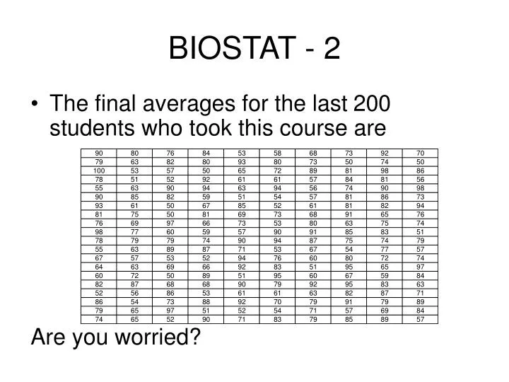
BIOSTAT - 2 • The final averages for the last 200 students who took this course are Are you worried?
BIOSTAT - 2 • Why not sort grades from highest to lowest [ordered array] • Is this a more meaningful way to present the data?
BIOSTAT - 2 • Why not group the data into grades of A, B, C, D, and F [frequency distribution] • That means we need to count the number of grades between 90 and 100, 80 and 89, etc. • Go to “Tools”, “Data Analysis (might have go to Tools, Add-Ins, and click on the 2 Data Analysis modules), Histogram, and follow directions.
BIOSTAT - 2 • Input range: sweep all your data • Bin range: sweep the cell boundaries you input somewhere on your spreadsheet – cell widths should normally be equal. • Now click on Cumulative % and Chart Output [this will plot your histogram] • OK
BIOSTAT - 2 • Output: • Histogram does not look right?
BIOSTAT - 2 • Fix histogram by eliminating gaps between cells. • Find “format data series” and “gap width”. How you do this depends on version of Excel you have. Note angle on labels for X-axis.
BIOSTAT - 2 • Unfortunately grades of 50 were not included in cells 50-59. That’s because Excel counts based on the following
BIOSTAT - 2 • Following bins seem to work
BIOSTAT - 2 • Final frequency table and histogram
BIOSTAT - 2 • Other statistical software will do the same thing, but you should always try out a small test case of data just to make sure that data is being placed into the proper cells.
BIOSTAT - 2 • Some key decisions: • How many cells should you have [we had 5 cells in this example]. In general, you would have between 5 and 25 cells. The more data you have, the more cells you would want to use. • How do you determine the Bin Ranges? Most statistical software will determine these bin ranges for you, but they might not be “neat” numbers. In this case, if you did not input specific bin ranges, you would get
BIOSTAT - 2 • Problems • Work problems 2.3.1and 2.3.5 • Look at data for problems 2.3.6 and 2.3.9
BIOSTAT - 2 • Numerical Techniques: • Measures of Central Tendency [Location] • Arithmetic Mean • Median • Mode • Measures of Dispersion [Variability] • Range • Variance • Standard Deviation
Measures of Central Location… • The arithmetic mean, a.k.a. average, shortened to mean, is the most popular & useful measure of central location. • It is computed by simply adding up all the observations and dividing by the total number of observations: Sum of the observations Number of observations Mean =
Arithmetic Mean… Sample Mean Population Mean
Measures of Central Location… • The median is calculated by placing all the observations in order; the observation that falls in the middle is the median. Data: {0, 7, 12, 5, 14, 8, 0, 9, 22} N=9 (odd) Sort them bottom to top, find the middle: 0 0 5 7 8 9 12 14 22 Data: {0, 7, 12, 5, 14, 8, 0, 9, 22, 33} N=10 (even) Sort them bottom to top, the middle is the simple average between 8 & 9: 0 0 5 7 8 9 12 14 22 33 median = (8+9)÷2 = 8.5
Measures of Central Location… • The mode of a set of observations is the value that occurs most frequently. • A set of data may have one mode (or modal class), or two, or more modes. If no values occur more than one time each, it is said that the data has no mode.
Measures of Variability… • Measures of central location fail to tell the whole story about the distribution; that is, how much are the observations spread out around the mean value? For example, two sets of class grades are shown. The mean (=50) is the same in each case… But, the red class has greater variability than the blue class.
Range… • The range is the simplest measure of variability, calculated as: • Range = Largest observation – Smallest observation • E.g. • Data: {4, 4, 4, 4, 50} Range = 46 • Data: {4, 8, 15, 24, 39, 50} Range = 46
Variance… • Variance and its related measure, standard deviation, are arguably the most important statistics. Used to measure variability, they also play a vital role in almost all statistical inference procedures. • Population variance is denoted by • (Lower case Greek letter “sigma” squared) • Sample variance is denoted by • (Lower case “S” squared)
Variance • Population Variance: • Sample Variance:
Sample Mean & Variance… Sample Mean Sample Variance Sample Variance (shortcut method)
Standard Deviation… • The standard deviation is simply the square root of the variance, thus: • Population standard deviation: • Sample standard deviation:
Excel Computations from Previous Data • Formulas: • Results: • Work Problem 2.5.7