Download
1 / 27
270 likes | 446 Views
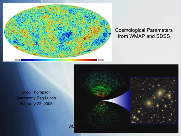
Observational constraints and cosmological parameters. Antony Lewis Institute of Astronomy, Cambridge http://cosmologist.info/. CMB Polarization Baryon oscillations Weak lensing Galaxy power spectrum Cluster gas fraction Lyman alpha etc…. +. Cosmological parameters.

E N D
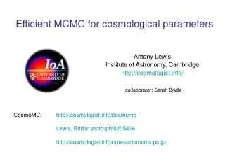
Observational constraints and cosmological parameters Antony Lewis Institute of Astronomy, Cambridge http://cosmologist.info/
CMB PolarizationBaryon oscillations Weak lensing Galaxy power spectrum Cluster gas fraction Lyman alpha etc… + Cosmological parameters
Bayesian parameter estimation • Can compute P( {ө} | data) using e.g. assumption of Gaussianity of CMB field and priors on parameters • Often want marginalized constraints. e.g. • BUT: Large n-integrals very hard to compute! • If we instead sample from P( {ө} | data) then it is easy: Use Markov Chain Monte Carlo to sample
Markov Chain Monte Carlo sampling • Metropolis-Hastings algorithm • Number density of samples proportional to probability density • At its best scales linearly with number of parameters(as opposed to exponentially for brute integration) • Public WMAP3-enabled CosmoMC code available at http://cosmologist.info/cosmomc (Lewis, Bridle: astro-ph/0205436) • also CMBEASY AnalyzeThis
WMAP1 CMB data alonecolor = optical depth Samples in6D parameterspace
Local parameters Background parameters and geometry • Energy densities/expansion rate: Ωm h2, Ωb h2,a(t), w.. • Spatial curvature (ΩK) • Element abundances, etc. (BBN theory -> ρb/ργ) • Neutrino, WDM mass, etc… • When is now (Age or TCMB, H0, Ωm etc.) Astrophysical parameters • Optical depth tau • Cluster number counts, etc..
General perturbation parameters -isocurvature- Amplitudes, spectral indices, correlations…
WMAP 1 CMB Degeneracies WMAP 3 All TT ns < 1 (2 sigma)
CMB polarization Page et al. No propagation of subtraction errors to cosmological parameters?
WMAP3 TT with tau = 0.10 ± 0.03 prior (equiv to WMAP EE) Black: TT+priorRed: full WMAP
ns < 1 at ~3 sigma (no tensors)? Rule out naïve HZ model
Secondaries that effect adiabatic spectrum ns constraint SZ Marginazliation Spergel et al. Black: SZ marge; Red: no SZ Slightly LOWERS ns
CMB lensing For Phys. Repts. review see Lewis, Challinor : astro-ph/0601594 Theory is robust: can be modelled very accurately
CMB lensing and WMAP3 Black: withred: without - increases ns not included in Spergel et al analysisopposite effect to SZ marginalization
LCDM+Tensors • No evidence from tensor modes • is not going to get much betterfrom TT! ns < 1 or tau is high or there are tensors or the model is wrong or we are quite unlucky So: ns =1
Other CMB: e.g. CBI combined TT data (Dec05,~Mar06) Thanks: Dick Bond
WMAP3WMAP3+CBIcombinedTT+CBIpol CMBall = Boom03pol+DASIpol +VSA+Maxima+WMAP3+CBIcombinedTT+CBIpol To really improve from CMB TT need good measurement of third peak
CMB Polarization Current 95% indirect limits for LCDM given WMAP+2dF+HST+zre>6 WMAP1ext WMAP3ext Lewis, Challinor : astro-ph/0601594
Polarization only useful for measuring tau for near future Polarization probably best way to detect tensors, vector modes Good consistency check
Matter isocurvature modes • Possible in two-field inflation models, e.g. ‘curvaton’ scenario • Curvaton model gives adiabatic + correlated CDM or baryon isocurvature, no tensors • CDM, baryon isocurvature indistinguishable – differ only by cancelling matter mode Constrain B = ratio of matter isocurvature to adiabatic -0.53<B<0.43 -0.42<B<0.25 WMAP1+2df+CMB+BBN+HST WMAP3+2df+CMB Gordon, Lewis:astro-ph/0212248
Degenerate CMB parameters Assume Flat, w=-1 WMAP3 only Use other data to break remaining degeneracies
Galaxy lensing • Assume galaxy shapes random before lensing Lensing • In the absence of PSF any galaxy shape estimator transforming as an ellipticity under shear is an unbiased estimator of lensing reduced shear • Calculate e.g. shear power spectrum; constrain parameters (perturbations+angular at late times relative to CMB) • BUT- with PSF much more complicated- have to reliably identify galaxies, know redshift distribution- observations messy (CCD chips, cosmic rays, etc…)- May be some intrinsic alignments- not all systematics can be identified from non-zero B-mode shear- finite number of observable galaxies
CMB (WMAP1ext) with galaxy lensing (+BBN prior) CFTHLS Contaldi, Hoekstra, Lewis: astro-ph/0302435 Spergel et al
Lyman alpha + WMAP WMAP 1 bfp: ns=0.97, s8=0.88 WMAP 3 (both +HST) Does not favour running: 0.005 ± 0.03 Ly-alpha: Viel Matteo, Haehnelt Martin G., Springel Volker, 2004, MNRAS, 354, 684
SDSS Lyman-alpha white: LUQAS (Viel et al)SDSS (McDonald et al) SDSS, LCDM no tensors: ns = 0.965 ± 0.015 s8 = 0.86 ± 0.03 ns < 1 at 2 sigma LUQAS
Conclusions • MCMC can be used to extract constraints quickly from a likelihood function • CMB can be used to constrain many parameters • Some degeneracies remain: combine with other data • WMAP3 consistent with many other probes, but favours lower fluctuation power than lensing, ly-alpha • ns <1, or something interesting • No evidence for running, esp. using small scale probes