Download
1 / 24
240 likes | 365 Views
Analysis of TowerA Van de Graff Data Instrument Analysis Workshop 6 SLAC February 27-28, 2006 Does the GLAST Monte Carlo successfully model real low energy photon data? Gary Godfrey godfrey@slac.stanford.edu. Introduction. VG proton beam hits a LiF target.

E N D
Analysis of TowerA Van de Graff Data Instrument Analysis Workshop 6 SLAC February 27-28, 2006 Does the GLAST Monte Carlo successfully model real low energy photon data? Gary Godfrey godfrey@slac.stanford.edu
Introduction • VG proton beam hits a LiF target. • Produces F(6.1), Li(14.6, 17.6) Mev photons (intensities.58 : .50 : 1.00) • Isotropic flux • Segmented (7 xtal x7 xtal) BGO calorimeter counts the number of photons entering a (3 xtal x 3 xtal) fiducial area.
BGO Monitoring BGO 3 x 3 fiducial volume spectrum for run VG112. Red= VG on. Blue= VG off for an equal amount of time. Cosmic peak ~120 MeV.
BGO Monitoring The blue points with error bars are the cosmic subtracted BGO 3 x 3 fiducial volume spectrum for run VG112. The black dots are a convolution of Gaussians and Lorentzians for the 3 lines using energies (7.1, 14.6, 17.6 Mev), intrinsic widths (.001, .01, 1.5 Mev), relative intensities (.58, .497, 1.00) , and a BGO energy σE/E = 13% at all energies.
BGO Monitoring • Simultaneously with a Tower A run, take a VGxxx run to measure the rate of F and Li [photons/sec] versus time in the BGO fiducial area. • # of photons produced / sterad = (Avrg rate in BGO) x (Sec of TowerA run) • MC Solid angle of BGO fiducial area • 3) MC Solid angle of BGO fiducial area = .102 .08 str
BGO Monitoring Cosmic subtracted, deadtime corrected F line rate (5-10 MeV summed) versus time for run VG112. Cosmic subtracted, deadtime corrected Li line rate (10-25 MeV summed) versus time for run VG112.
TowerA Trigger Rates • There were 12 – one hour front face E2E and SVAC runs, various configurations, VG ON. For each run: • Calculate the deadtime corrected trigger rate. • Subtract the cosmic ray rate of Run 135000954. • Measure the F and Li photon rates using the BGO. • Predicted trigger rate= • ( MC EfficΩtower x BGO rate)F + ( MC EfficΩtower x BGO rate)Li MC Ωbgo MC Ωbgo • The Tower is much less efficient for triggering on F than Li photons. • MC EfficΩtower(F)= .028 str MC EfficΩtower(Li)=.348 str • Calculate Ratio= Measured Trig Rate / Predicted Trig Rate • The average Ratio was 1.10 .05 statistical varience of 12 runs • .08 systematic BGO distance error
Run 135000949 • Horizonal LAT 1” in front of VG target. LAT z axis parallel to VG pipe. • VG is ON. BGO run VG112. Tower run 135000949. • Events are used in the following plots if GoodTrk= .True. • GoodTrk = [Vtx1NumTkrs ≥ 1] At least 1 track • and [Tkr1NumHits ≥ 4] Looser than 6 hit hardware trigger • and [abs(VtxX0+560.) ≤ 250.] Vertex in loose Tower volume • and [abs(VtxY0+560.) ≤ 250.] • and [0. < VtxZ0 < 610.]
Run 135000949 MC data tracks extrapolated to a plane 40 mm in front of the top silicon layer. VG data tracks extrapolated to a plane 40 mm in front of the top silicon layer. Fraction of hits in a 60 mm diameter circle centered on the spot versus the distance of the extrapolation plane from the top silicon. MC (red histogram), VG (black points), and Cosmics (blue histogram)
VG & Cosmics: Cos Distributions by Layer The black histograms are VG cos (between the track and the z axis of the tower) distributions. The blue curves are cosmic data. Each plot is for tracks with their vertex in a particular layer. Cut1=Top most gap of tower. Cut18=Bottom most gap of tower.
VG & MC:Cos Distributions by Layer The black histograms are VG-cosmics cos (between the track and the z axis of the tower) distributions. The red histograms are the MC. Cut1=Top most gap of tower. Cut18=Bottom most gap of tower.
(VG-Cosmics) & MC :Track Vertex Distribution in X by Layer Number of track origins versus transverse position x. The black histograms are VG-Cosmics and the red histograms are MC.
(VG-Cosmics) & MC :Track Vertex Distribution in Y by Layer Number of track origins versus transverse position y. The black histograms are VG-Cosmics and the red histograms are MC.
Distribution of Track Vertices in Z The number of track origins as a function of z. ( Log scale and Linear scale). The black points with statistical error bars are the VG data. The red is the MC. VG/MC= .83 (bottom layers) =.92 (middle layers =1.06 (top layers) 0% 18%3% Tungsten radiators | | | | | | | | | | | | | | | | | |
Energy Deposited in Cal vs Vertex Layer Energy deposition in the calorimeter for tracks originating in different layer. The black histogram is VG-cosmics and the red histogram is MC. Cut16 is the pair of silicon layers with the bottom most super GLAST radiator.
Tower PSF for VG Photons • The cos distribution between the track unit vector and a line drawn from the vertex to the target center. The black histogram is the VG-cosmic data and the red curve is the MC. • The integral of the cos distributions are shown in (a). From plot (b) one reads off cos(68)=.83 and .86 for VG data and MC. • (a) (b)
LAT VG Run • Goal: Compare the low energy g acceptance of the final LAT to the MC with only a few percent normalization error. • Parasitic to SVAC Horiz LAT Cosmic data taking. • VG on during ~5 hrs of the ~15 hrs of Horiz LAT Cosmic Run. • Adds ~5 Hz to the ~250 Hz LAT trig rate. • Systematic error on normalization will be smaller, since absorption of target window and Pb will be the same for BGO and LAT. • Target will appear to the LAT as an “AGN” point source that must be separated from the ~50 times larger bkgnd of charged cosmics (and ~5 times larger bkgnd of cosmic shower photons).
Summary • Known numbers of F(6.1) + Li(14.6+17.6) Mev photons generated by a Van de Graaff accelerator and by a Monte Carlo were put into Tower A. • Measured trigger rates for 12 runs were 1.10 times that expected from MC. This is consistent with an estimated .08 systematic error from the BGO monitoring used to scale the MC. • For the one run compared in detail to the MC, the number of “GoodTrk” VG events was 1.07 times that expected from the MC. (Approx the same 1.10 factor seen in the trigger rates). • After removing the 1.07 normalization factor: • The distribution of track vertices in cos , x, y, and z show agreement between VG data and MC. • For vertices in the bottom two super Glast layers, the energy reaching the cal shows agreement in shape between the VG data and MC. However, the number of cal events for the VG data is low by ~2 compared to the MC.
Summary • There is reasonable agreement between the real data and MC PSF for the VG energy photons. The MC is slightly broader than the data at small angles, and has a slightly lower tail than the data at big angles. This results in cos(68)=.83 (68=34) and .86 (68=31) for VG data and MC. The target half width is σtarget ~ (.75”/2.0”) x (180/p) = 21°, which must be subtracted in quadrature from 68 to obtain the actual tower PSF. • The next comparisons between calibrated sources of photons and the GLAST MC will be: • VG photons into the full LAT (target ~10 feet from LAT at ~37°) • Brems photons into the 2-Tower Calibration Unit at CERN
Tower PSF for VG Photons • The VG target is only 1” from the front face of the tower. • Therefore, the cos (between the track and the z axis of the tower) distribution is very broad (eg: tracks which point at the target for a vertex at the edge of the tray have very different cos than a vertex in the center of the tray). • So, attempt to measure the Tower PSF by plotting the cos distribution between the track unit vector and a line drawn from the track vertex to the target center. • This width of this distribution will be a convolution of the true Tower PSF and the VG LiF target size. The target half width is qtarget ~ (.75”/2.0”) x (180/p) = 21°, which must be subtracted in quadrature from the measured 68 to obtain the actual tower PSF. • The plot on the next transparency shows: cos(68)=.83 • 68 =34° • PSF =sqrt(342-212)=26°
VG Xray Bursts (135000949 1/8” Pb) Number of Events vs. Number of strips Trans(1/8” Pb, 200 Kev)=.03 Layer 18 x,y Layer 16 x,y Layer 14 x,y