Download
1 / 10
100 likes | 176 Views
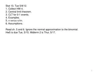
Stat 13, Thu 5/10/12. 1. CLT again. 2. CIs. 3. Interpretation of a CI. 4. Examples. 5. Margin of error and sample size. 6. CIs using the t table. 7. When to use z* and t*. Read ch. 5 and 6. Hw5 is due Tue, 5/15. Midterm 2 is Thur, 5/17.

E N D
Stat 13, Thu 5/10/12. 1. CLT again. 2. CIs. 3. Interpretation of a CI. 4. Examples. 5. Margin of error and sample size. 6. CIs using the t table. 7. When to use z* and t*. Read ch. 5 and 6. Hw5 is due Tue, 5/15. Midterm 2 is Thur, 5/17. On Thur, 5/17, I won’t be able to have my usual office hour from 230 to 3:30, so it will be instead from 1:30 to 2:15pm.
1. Central Limit Theorem (CLT). If you have a SRS (or observations are iid), and n is large (or the population is normally distributed), then is normally distributed with mean µ and std deviation , where s is the std deviation of the population and n is the sample size.
2. CIs. The examples from last class were a little artificial, because we KNEW the population mean µ. Usually you take a sample because you don't know µ. We then use the sample mean to estimate the population mean µ. But what if we want a range, or interval, where we think µ is likely to fall, based on ? That's called a confidence interval (CI). We know from the CLT that is normally distributed with mean µ and std deviation . This means the difference between and µ is typically around . So from this info, we can tell given where µ seems likely to lie. For instance, if we know = 10, and = 1, then it seems pretty likely that µ is between 9 and 11, and very likely between 8 and 12. The way to get a c%-confidence interval using the Z table: * First find the values from the table that contain the middle c% of the area under the standard normal curve. If c = 95, that means 2.5% is to the right of the region, and 2.5% (0.025) is to the left, so you look in Table A til you find 0.025 and you see the appropriate value is 1.96. We call this z* = 1.96. (or see bottom row of table 4 or in back of book: 95% corresponds to 1.96. 80% would correspond to 1.282.)
The way to get a c%-confidence interval using the Z table: * First find the values from the table that contain the middle c% of the area under the standard normal curve. If c = 95, that means 2.5% is to the right of the region, and 2.5% (0.025) is to the left, so you look in Table A til you find 0.025 and you see the appropriate value is 1.96. We call this z* = 1.96. (or see bottom row of table 4 or in back of book: 95% corresponds to 1.96. c = 80 would correspond to z* = 1.282.) * Now, just use the formula: +/- z* , and you have your CI. For a different confidence level besides 95%, the value of z* would change. The use of this formula is based on the CLT. It can only be used if the following assumptions are met: (i) SRS (or somehow you know that the observations are iid), AND (ii) n is large (or population is ~ normal and s is known). Typically you don't know s. If n is large you can just plug in s, the standard deviation of the observations in your SAMPLE. In the case of 0-1 data, s = , where and are the proportion of 0's and 1's in the sample.
3. Interpretation of a 95% CI: there's a 95% chance that the CI contains the true population mean µ. The CI is a random variable (statistic, estimate): If another sample were taken, there'd be a different sample mean , and therefore a different CI. Unless we're really unlucky, our CI will contain µ. That is, if we kept sampling over and over, and each time we got a different and a different 95%-CI, then 95% of these CIs would contain µ. 4. Examples. Suppose we don't know the mean amount of wet manure produced by the avg cow. We sample 400 cows and find that in our sample, the mean is = 18 pounds, and the sample standard deviation is s = 5 pounds. Find a 92%-CI for the population mean. Answer: It’s a SRS and n = 400 is large, so the standard formulas apply, but we don’t know s so we will plug in s. For a 92%-CI, we want the values containing 92% of the area, which means 4% is to the right and 4% is to the left, so from the table, z* = 1.75. The CI is +/- (z*)s/√n = 18 +/- (1.75)(5) ÷ √400 = 18 +/- 0.4375.
Another example. Suppose we don't know the percentage of people with peanut allergies. We take a SRS of 900 people. We find that 72 of them (8.0%) of them have peanut allergies. Find a 90%-CI for the population percentage of people with peanut allergies. Answer: This is a 0-1 question. It’s a SRS and n is large because there are 72 with allergies and 828 without, and both of these are ≥ 10. So the standard formulas apply. For a 90%-CI, z* = 1.645 from the bottom row of Table 4. The formula for the 90%-CI is +/- z* s/√n. We don't know s so use s = = √ (8.0% x 92.0%) ~ 0.271. Our 90%-CI is 8.0% +/- (1.645) (0.271) / √900 which is 8.0% +/- 1.486%. 5. Margin of error and sample size. This +/- part is called a margin of error.
5. Margin of error and sample size. This +/- part is called a margin of error (m in the book). m = z* s/√n. Suppose you know what margin of error, m, you want. But you don't know what sample size n you need. Just let m = z* s/√n. Solving for n, we get n = (z* s / m)2. This tells you how large the sample size needs to be to achieve the margin of error. Typically for margin of error you want a 95%-confidence level, so z* = 1.96, unless otherwise specified. Example: Continuing with peanut allergies, we took a SRS of 900 people and found that 72 of them (8.0%) of them had peanut allergies and a 90%-CI for the population percentage of people with peanut allergies was 8.0% +/- 1.486%. How many more people are needed to get this margin of error for the 90%-CI down to 1%? Answer: n = (z* s / m)2. Here it’s a 90%-CI so z* = 1.645. s is unknown so use s = √ (8.0% x 92.0%) ~ 0.271. m = 1%. So, n = (1.645 x 0.271 / .01)2 ~ 1987. We already have 900 so we need 1087 more.
6. Using the t table. Assumptions for CIs using the Z (std normal) table: (i) SRS (or somehow you know that the observations are iid), AND (ii) n is large (or the population is normal and s is known). Under these conditions, the CLT says that is normally distributed with mean µ and std deviation , so a CI is +/- z* , and you can substitute s for s. If n is small and you know the population is normal, then s might be substantially different from s. If s is unknown but estimated using s, then use of the t table is appropriate, rather than the Z table. Specifically, if you have: (i) SRS (or the observations are iid), AND (ii) population is normal, AND (iii) s is unknown, and estimated with s, then is tn-1 distributed with mean µ and std deviation , so a CI is +/- t* s/√n. t* is given in Table 4 or the back of the book. n-1 is the “degrees of freedom” (df). Can't use the Z table when n is small and distribution of the population is unknown.
Example using the t table. Suppose you take a SRS of 10 patients with hand, foot and mouth disease and record their ages. You find that is 12 and s = 7. Find a 95% CI for µ, the mean age among the whole population of patients with hand, foot and mouth disease, assuming the ages in this population are normally distributed. Answer. Here we have a SRS, the pop. is normal, and s is unknown, so use the t table. df = n-1 = 10-1 = 9. From Table 4, for a 95% CI, with df = 9, t* = 2.26. So, the 95% CI is +/- t* s/√n = 12 +/- 2.262 (7)/√10 = 12 +/- 5.01, or the interval (6.99,17.01). Note that if the population is 0s and 1s, then this contradicts the assumption that the population is normal, so you’d never use the t table with this type of data.
7. When to use z* and t*. The book seems to always recommend using t* rather than z*. a) If it's a simple random sample (SRS) and the population is normal, s is unknown, and n is small (< 25), then use t*. b) If it's a SRS and the population is normal, s is known, and n is small (< 25), then use z*. c) If it's a SRS and n is large, then t* and z* are very close together, so it doesn't really matter which you use. The book recommends t*, but I'm going to suggest you use z* since it's easier to determine, especially when the sample size is such that the df isn't a value in the table on the last page of the book. On the hw, I will tell the reader to accept either t* or z* for this case, and similarly on my exams. d) One thing that's crucial to me is that you understand that, if the population might NOT be normal and n is NOT large, then neither t* nor z* is appropriate.