Download
1 / 8
80 likes | 180 Views
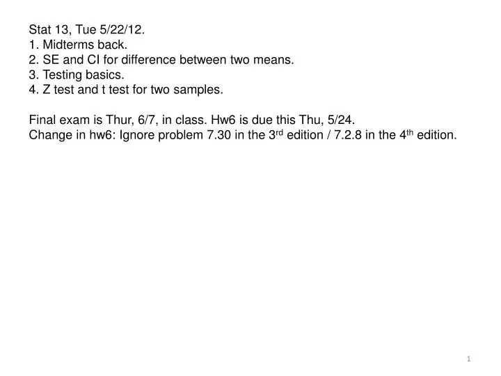
Stat 13, Tue 5/22/12. 1. Midterms back. 2. SE and CI for difference between two means. 3. Testing basics. 4. Z test and t test for two samples. Final exam is Thur, 6/7, in class. Hw6 is due this Thu, 5/24. Change in hw6: Ignore problem 7.30 in the 3 rd edition / 7.2.8 in the 4 th edition.

E N D
Stat 13, Tue 5/22/12. 1. Midterms back. 2. SE and CI for difference between two means. 3. Testing basics. 4. Z test and t test for two samples. Final exam is Thur, 6/7, in class. Hw6 is due this Thu, 5/24. Change in hw6: Ignore problem 7.30 in the 3rd edition / 7.2.8 in the 4th edition.
Be SILENT while I am passing out the exams or I will ask you to leave. Gradegrubbing procedure, again: if you would like a question (or more than one question) reevaluated, submit your exam or homework and a WRITTENexplanation of why you think you deserve more points and how many more points you think you deserve to your TA. The TA will then give it to me, and I will consider it, and then give it back to the TA to give back to you. Midterms: 90-100 = A range, 80-90 = B range, 70-80 = C range, 60-70 = D range, < 60 = F. I record your number, not the letter grade. Your grade is on the last page. Mean = 83. SD = 19. Common things: * 2. 95% of the values for the normal distribution are in µ +/- 1.96 s. 1.96(5.2) ~ 10.2. * 8. I messed up here and said rabbit lengths instead of rabbit hair counts. * 14. Let X1 = 1 if the 1st sample mean is < 102.4, and 0 otherwise. Similarly for X2 and X3. X = X1 + X2 + X3. E(X) = E(X1) + E(X2) + E(X3) = 88.49% + 88.49% + 88.49% ~ 2.655. * Do not guess NOTA. I never, ever intend for the correct answer to be NOTA. So, if you’re getting an answer that is not there, check to see if you’ve made a mistake.
2. SE and CI for difference between two means. Suppose you have two samples: a SRS of size n1 from population 1 and a SRS of size n2 from population 2. For instance, pop. 1 is those drinking 4-6 cups of coffee daily, and pop. 2 is those drinking 0 cups a day. For each person, record blood pressure (BP). Let µ1 be the mean BP of population 1, and µ2 is the mean BP of population 2. Let 1 be the mean BP of sample 1, and 2 is the mean BP of sample 2. Often we’re interested in estimating the difference, µ1 - µ2. Our estimate would be 1 - 2. But what if we want a 95% CI for µ1 - µ2? We’d simply use be 1 - 2 +/- 1.96 SEdiff, where SEdiff is the standard error for the difference, i.e. the typical distance between the difference between sample means and the difference between the two pop.means. There’s an easy formula. SEdiff = √ (SE12 + SE22), where SE1 = is the SE for sample mean 1 and SE2 = is the SE for sample 2. So SEdiff = √ (SE12 + SE22) = √(s12/n1 + s22/n2). Usual CLT assumptions must hold for both samples, and if n is large, plug in s for s. For example, suppose sample 1 is an SRS of 100 coffee drinkers, and in this sample, 1 = 124 and s1 = 10. Sample 2 is an SRS of 85 non-drinkers, and 2 = 127, s2 = 8. Then a 95% CI for µ1 - µ2 would be 1 - 2 +/- 1.96 SEdiff, which is 124 - 127 +/- 1.96 √(102/100 + 82/85) = -3 +/- 2.60. Note: it doesn’t cover 0.
If both populations are known to be normally distributed, and n1 and n2 are small, and they’re both SRSs, then you’d substitute z* = 1.96 (for a 95% CI) for t*, where now the degrees of freedom, df = n1 + n2 – 2. Ignore Formula 6.7.1 on p227 in the 3rd edition = Formula 7.1 in the 4th edition, involving the df for the difference between two means. Use n1 + n2 - 2 instead. A 95% CI for µ1 - µ2 would be 1 - 2 +/- t* SEdiff. For instance, with all the numbers the same as in the last example, but if both populations were known to be normally distributed, and n1 = 10 and n2 = 7, df = 17-2 = 15, so t* = 2.131, and now SEdiff = √(102/10 + 82/7) = 4.375, and a 95% CI for µ1 - µ2 would be 124 - 127 +/- 2.131(4.375) = -3 +/- 9.323. The exact same formula holds when both samples are of 0-1 data. For instance, say you record 1 if the person dies and 0 if he/she survives the 15 year period. In the SRS of 100 coffee drinkers, 18% die, and in the SRS of 85 nondrinkers, 23% die. A 95% CI for the difference between the two population percentages is... 18% - 23% +/- 1.96 √(s12/n1 + s22/n2), [s1 = √(18% x 82%), so s12 simply = 18% x 82%] = -5% +/- 1.96 √(18% x 82%/100 + 23% x 77%/85) = -5% +/- 11.69%. So, this time it contains 0, so we can’t rule out the possibility that there is no difference between the two population percentages. That is, the difference between the two sample percentages might be due to chance alone.
3. Testing basics. Suppose you take two SRSs from two populations and you want to test whether the population means might really be the same. e.g. one sample mean = 18% and the other is 23%. You want to test whether something like this could reasonably have happened just by chance alone, if the populations were actually identical. Otherwise we conclude that the two population means are probably not equal. There are different tests, but we’ll just talk about the Z-test (or normal test) and t test. Assumptions: same as before. For each sample, it must be SRS (or obs are known to be independent) AND n is large (or pop is known to be normally distributed). If in addition, for at least one of the samples, n is small, pop. is normal, and s is unknown, then use t instead of Z. After checking assumptions, the remaining steps in testing are * stating the hypotheses, * computing the test statistic (Z or t), * computing the p-value, and * concluding.
Hypotheses. Let µ1 and µ2 be the means of the populations from which the samples are drawn. Null hypothesis (Ho): µ1 = µ2. This means that the observed difference between 1 and 2 is due to chance alone. Alternative hypothesis (Ha): µ1 ≠ µ2. Difference is not due to chance alone. (2-sided test.) Or Ha: µ1 > µ2. Or Ha: µ1 < µ2. (1-sided tests). Direction depends on your data. When in doubt, do a two-sided test, unless I specifically say to do a 1-sided test. Usually we specify these hypotheses numerically. Z-statistic. A test statistic is a summary of the data. Z-statistic =( 1 -2) ÷ SEdiff. Same for t, but call it t! If either s is unknown, just plug in s. P-value. The p-value is the probability, assuming Ho is true, that the test statistic will be at least as extreme as that observed. Use normal table, or with the t table, figure out if the t-statistic is bigger than the critical value t* for your corresponding value of a, which is the significance level of the test (typically a is 5%). For a one-sided test, cut the p-value in half. Conclusion. Small p-value = strong evidence against Ho. Large p-value = weak evidence against Ho. The observed difference is statistically significant if the p-value < 5%. The observed difference is highly significant if the p-value < 1%.
Examples. Again, suppose sample 1 is an SRS of 100 coffee drinkers, and in this sample, 1 = 124 and s1 = 10. Sample 2 is an SRS of 85 non-drinkers, and 2 = 127, s2 = 8. Do a test at significance level a = 5% to see if the two sample means are significantly different. Check assumptions. Both SRSs and n is large in each. Ho: µ1 = µ2. Ha: µ1 ≠ µ2. (two-sided). If one-sided, it’d be Ha: µ1 < µ2. z =( 1- 2) ÷ SEdiff = (124-127) ÷ √(102/100 + 82/85) = -3 ÷ 1.324 = -2.27. So, the p-value for this 2-sided test is P(std normal is < -2.27) + P(std normal is > 2.27) = 2 x 0.0116 =.0232 = 2.32%. The p-value is smaller than 5%, so the difference is statistically significant. This means the evidence against the null hypothesis is strong, i.e. we have strong evidence suggesting that coffee drinkers and non coffee drinkers have different average BPs. The difference (between the sample means of 124 and 127) is statistically significant, and is very unlikely to be due to chance alone. Note that sample size is a factor. Sometimes a difference of -3 is statistically significant, and sometimes it’s not. It depends on the sample size and the SDs.
An example using t, and where the first sample mean is bigger, and where it’s not stat. sig. Suppose sample 1 is an SRS of 10 coffee drinkers, and in this sample, 1 = 127 and s1 = 10. Sample 2 is an SRS of 8 non-drinkers, and 2 = 124, s2 = 7. Both populations are normal. Do a test at significance level a = 5% to see if the two sample means are significantly different. Check assumptions. Both SRSs, pops are normal, n is small, ss are unknown, so do a t test. Ho: µ1 = µ2. Ha: µ1 ≠ µ2. (two-sided). If one-sided, we would write Ha: µ1 > µ2. t =( 1- 2) ÷ SEdiff = (127-124) ÷ √(102/10 + 72/8) = 3 ÷ 4.016 = 0.747. Using the t-table, we can’t figure out the exact p-value for this test but we can find the critical value t*. df = n1 + n2 - 2 = 16, and a = 5% so t*16 = 2.120. Our observed t = 0.747. If our t = 2.120, then our p-value would be 5%. If our t > 2.120, then our p-value would be < 5%. Here, our t < 2.120, so our p-value is > 5%. This means that the observed difference is not statistically significant. The evidence is weak against the null hypothesis that coffee drinkers and non coffee drinkers have the same average BPs. The difference (between the sample means of 127 and 124) is not statistically significant, and could plausibly be attributed to chance alone.