Download
1 / 62
630 likes | 658 Views
Explore basic robotics concepts in mechanics, control theory, and computer science. Hands-on experiments with LEGO Mindstrom Kit and robotic arm. Design and build a wheeled robot from scratch. Course materials, requirements, evaluation, grading outlined.

E N D
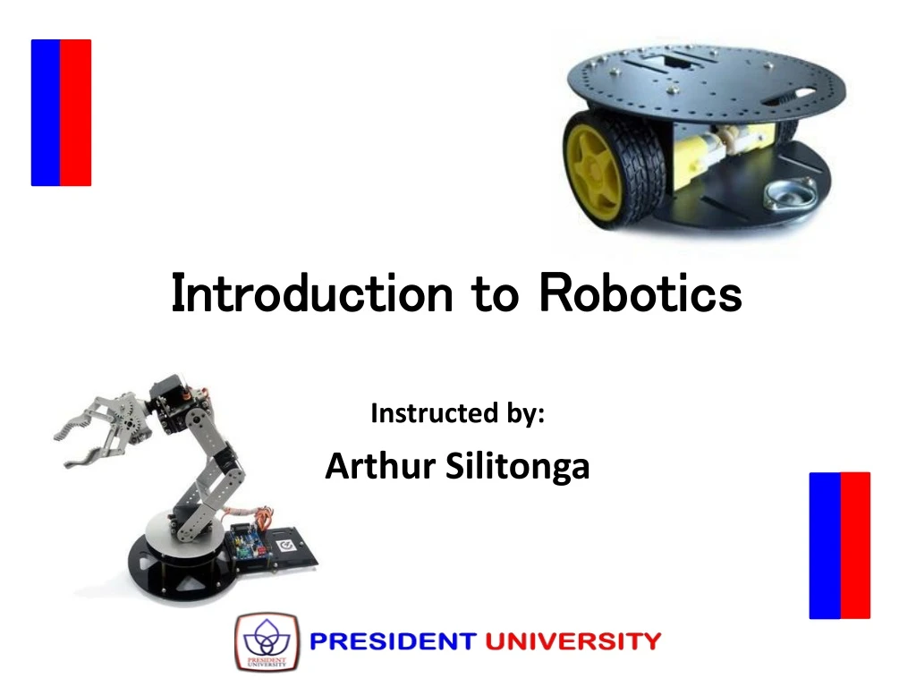
Introduction to Robotics Instructed by: Arthur Silitonga
Outline • Course Information • Course Overview & Objectives • Course Materials • Course Requirement/Evaluation/Grading (REG)
I. Course Information • Instructor + Name : Arthur Silitonga + Address : Jl. Ki Hadjar Dewantara, President University, Cikarang, Bekasi + Email Address : arthur@president.ac.id + Office Hours : Tuesday, 17.00 – 18.00 • Course‘s Meeting Time & Location + Meeting Time : Tuesday -> 10.30 – 13.00 (Lec) : Friday -> 07.30 – 10.00 (Lab) + Location : Room B, President University, Cikarang Baru, Bekasi
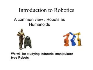
II. Course Overview & Objectives • Lecture sessions are tightly focused on introducing basic concepts of robotics from perspectives of mainly mechanics, control theory, and computer science. • Experiments at the lab occupying LEGO Mindstrom Kit, Wheeled Robot, and Robotic Atm. • Students are expected to design and implementing a real wheeled robot “from the scratch“. Course Overview
Course Objectives The objectives of this course are students should be able to : • describe positions and orientations in 3-space mathematically, and explain the geometry of mechanical manipulators generally • acquire concept of kinematics to velocities and static forces, general thought of forces & moments required to cause a motion of a manipulator, and sub-topics related to motions & mechanical designs of a manipulator • recognize methods of controlling a manipulator, and simulate the methods during lab works concerning to concepts of Wheeled Robot and Robotic Arm • design a wheeled robot “from the scratch“ based on knowledge of mechatronics To accomplish the objectives students will : • have homework assignments and participate in quizzes • implement calculations of 3-space positions & orientations using LEGO Mindstrom kit • design a wheeled robot considerating to theoretical and practical aspects • implement software aspects of a robotic arm • should take the mid-term exam, and the final exam
IV. Course Requirement/Evaluation/Grading • Requirements : - physics 1(mechanics) - linear algebra (matrix and vector) • Evaluation for the final grade will be based on : - Mid-Term Exam : 30 % - Final Exam : 30 % - Lab Experiments or Assignments : 20 % - Course Project : 20% Every two weeks, a quiz will be given as a preparation of several lab experiments
Mid-Term Exam consists of Lectures given in between the Week 1 and the Week 6. • Final Exam covers whole subjects or materials given duringthe classes. • Grading Policy Final grades may be adjusted; however, you are guaranteed the following: If your final score is 85 - 100, your grade will be A. If your final score is 70 - 84, your grade will be B. If your final score is 60 - 69, your grade will be C. If your final score is 55 - 59, your grade will beD. If your final score is < 55, your grade will be E.
REFERENCES • [Cra05]Craig, John., Introduction to Robotics : Mechanics and Control(Third Edition). Pearson Education, Inc.: New Jersey, USA. 2012. • [Sie04] Siegwart, Roland. & Nourbakhsh, Illah., Introduction to Autonomous Mobile Robots. The MIT Press : Cambridge, USA. 2004. • [Sic08]Siciliano, Bruno. & Khatib, Oussama., Handbook of Robotics. Springer-Verlag: Wuerzburg, Germany. 2008. • [Do08]Dorf, Richard. & Bishop, Robert., Modern Control Systems (Eleventh Edition). Pearson Education, Inc: Singapore, Singapore. 2008.
Contents • Acceleration & Mass Distribution • Newton‘s equation and Euler‘s equation • Iterative Newton – Euler Dynamic Formulation • Structure of A Manipulator‘s Dynamic Equ. • Lagrangian Formulation • General Description in Path Descriptions & Generation • Joint-Space Schemes • Cartesian-Space Schemes
Basing the Design on Task Requirements • Kinematic Configuration • Quantitative Measures • Redundant and Close-Chain Structures • Actuator Schemes • Stiffness and Deflections • Position Sensing • Force Sensing
AccelerationandMass Distribution • We have studied static positions, static forces, and velocities; but we have never considered the forces required to cause motion. • In this part, we consider the equations of motion for a manipulator. • The way in which motion of the manipulator arises from torques applied by the actuators or from external forces applied to the manipulator.
There are two problems related to the daynamics of a manipulator that we wish to solve. - first problem, given a trajectory point, , , and we wish to find the required vector of joint torques, r. - second problem, calculating how the mechanism will move under application of a set of joint torques. This case indicates that there is a a torque vector, r, and we need to calculate the resulting motion of the manipulator , , and .
Acceleration of a Rigid Body • We extend our analysis of rigid-body motion to the case of accelerations. • At any instant, the linear and angular velocity vectors have derivatives that are called the linear and angular accelerations, respectively. and Linear Acceleration
As with velocities, when the reference frame of the differentiation is understood to be some universal reference frame, {U}, the notation is • The velocity of a vector as seen from frame {A} when the origins are coincident :
Expressing the acceleration of as viewed from {A} when the origins of {A} and {B} coincide : • Combining the two terms :
Finally, to generalize to the case in which the origins are not coincident, we add one term which gives the linear acceleration of the origin of {B}, resulting in the final general formula : When
Angular Acceleration Consider the case in which {B} is rotating relative to {A} with AQB and {C} is rotating relative to {B} with By differentiating, we obtain
Mass Distribution • In systems with a single degree of freedom, we often talk about the mass of a rigid body. • In the case of rotational motion about a single axis, the notion of the moment of inertia is a familiar one. • We introduce the inertia tensor, which, for our purposes, can be thought of as a generalization of the scalar moment of inertia of an object.
Figure 13.1 The inertia tensor of an object describes the object's mass distribution. The vector AP locates the differential volume element Δv
For a rigid body that is free to move in three dimensions, there are infinitely many possible rotation axes. • The inertia tensor relative to frame {A} is expressed in the matrix form as the 3 x 3 matrix
In which the rigid body is composed of differential volume elements, dv, containing material of density ρ. • Each volume element is located with a vector • The elements Ixx, Iyy, and Izz are called the mass moments of inertia. • The elements with mixed indices are called the mass products of inertia.
This set of six independent quantities depend on the position and orientation of the frame in which they are defined. • If we are free to choose the orientation of the reference frame, it is possible to cause the products of inertia to be zero. • A well-known result, the parallel-axis theorem, is one way of computing how the inertia tensor changes under translations of the reference coordinate system. • The parallel-axis theorem relates the inertia tensor in a frame with origin at the center of mass to the inertia tensor with respect to another reference frame.
Where {C} is located at the center of mass of the body, and {A} is • an arbitrarily translated frame, the theorem can be stated as
Newton‘sEquation, andEuler‘sEquation • Newton's equation, along with its rotational analog, Euler's equation, describes how forces, inertias, and accelerations relate. Fig. 13. 2 A force F acting at the center of mass of a body causes the body to accelerate at
where m is the total mass of the body. • a rigid body rotating with angular velocity ω and • with angular acceleration . • The moment N, which must be acting on the body • to cause this motion, is given by Euler's equation
Fig. 13.3 A moment N is acting on a body, and the body is rotating with velocity ω, andaccelerating at
Iterative Newton-Euler Dynamic Formulation • We assume we know the position, velocity, and acceleration of the joints ( , , ). • With this knowledge, and with knowledge of the kinematics anf the mass-distribution information of the robot, we can calculate the joint torques required to cause this motion.
Outward iterations to compute velocities and accelerations • The force and torque acting on a link • Inward iterations to compute forces and torques • The iterative Newton-Euler dynamics algorithm • Inclusion of gravity foces in the dynamics algorithm
The Iterative Newton-Euler Dynamics Algorithm • The complete algorithm for computing joint torques from the motion of the joints is composed of two parts. First, link velocities and accelerations are iteratively computed from link 1 out to link n and the Newton—Euler equations are applied to each link. • Second, forces and torques of interaction and joint actuator torques are computed recursively from link n back to link 1.
Trajectory : a time history of position, velocity, and acceleration for each degree of freedom. • Concept of creating trajectory : - specification - representation - generation
General Considerations In Path Description and Generation • Consider motions of a manipulator as motions of the toolf frame {T}, relative to the station frame, {S}. • Idea : move the manipulator from an initial position to some desired final position.
Designing a path description : give a sequence of desired via points (intermediate points between the initial and final positions). • Each of the via points is actually a frame that specifies both the position and orientation of the tool relative to the station. • Path points : via points, initial and final points.
Joint-Space Schemes • The path shapes (in space and in time) are described in terms of functions of joint angles. • Each path point is isually specified in terms of a desired position and orienation of the tool frame {T}, relative to the station frame, {S}. • Joint-space schemes achieves the desired position and orientation at the via points.
Initial position of the manipulator is also known in the form of a set of joint angles. • tO is the initial position of the joint, and tf is the desired goal position of that joint. • There are some funtions which might be used to interpolate the joint value. Cubic polynomials
These four constraints can be satisfied by a polynomial of at least third degree. so the joint velocity and acceleration along this path are clearly
Cubic Polynomials For A Path With Via Points Fig.13.4 Position Fig. 13.5 Velocity
Higher-order polynomials • if we wish to be able to specify the position, velocity, and acceleration at the beginning and end of a path segment, a quintic polynomial is required, namely