Download
1 / 16
160 likes | 167 Views
Tomasz Czarski W arsaw U niversity of T echnology Institute of Electronic Systems ELHEP-DESY Group. Superconductive cavity driving with FPGA controller. Main topics. Low Level RF control system introduction Superconducting cavity modeling Cavity features

E N D
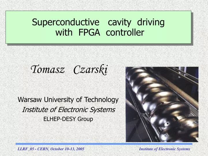
Tomasz Czarski Warsaw University of Technology Institute of Electronic Systems ELHEP-DESY Group Superconductive cavity driving with FPGA controller
Main topics • Low Level RF control system introduction • Superconducting cavity modeling • Cavity features • Recognition of real cavity system • Cavity parameters identification • Control system algorithm • Experimental results
CAVITY RESONATORandELECTRICFIELD distribution FIELD SENSOR COUPLER KLYSTRON CAVITY ENVIRONS ANALOG SYSTEM PARTICLE DOWN-CONVERTER 250 kHz MASTER OSCILATOR 1.3 GHz VECTOR MODULATOR FPGA I/Q DETECTOR FPGA CONTROLLER DAC ADC DIGITAL CONTROL SYSTEM CONTROL BLOCK PARAMETERS IDENTIFICATION SYSTEM Functional block diagram of Low Level Radio Frequency Cavity Control System
CAVITY transfer function Z(s) = (1/R+ sC+1/sL)-1 RF voltage Z(s)∙I(s–iωg) RF current I(s–iωg) Analytic signal: a(t)·exp[i(ωgt + φ(t))] Demodulation exp(-iωgt) Modulation exp(iωgt) Complex envelope: a(t)·exp[iφ(t)] = [I,Q] Low pass transformation Z(s+iωg) ≈ ω1/2·R/(s +ω1/2–i∆ω) half-bandwidth = ω1/2 detuning = ∆ω Input signal I(s)↔i(t) Output signal Z(s+iωg)∙I(s)↔v(t) State space – continuous and discrete model vn = E·vn-1+ T·ω1/2·R·in-1 E = (1-ω1/2·T) + i∆ω·T dv/dt = A·v + ω1/2·R·i A = -ω1/2+i∆ω Superconductive cavity modeling
Particle Field sensor Coupler Cavity features Cavity parameters: resonance circuitparameters: R L C
Internal CAVITY model Internal CAVITY model Internal CAVITY model Output distortion factor Input distortion factor vk = Ek-1·vk-1 + uk-1 - (ub)k-1 E = (1-ω1/2·T) + i∆ω·T D C v u + u0 CAVITY environs Input offset phasor Input offset compensator + u’0 C’ Output calibrator FPGA controller area Input calibrator D’ Output phasor v’ External CAVITY model v’k = Ek-1·v’k-1 + C·C’·D·[D’·u’k-1 + u’0 + u0)] – C·C’·(ub)k-1 u’ Input phasor Algebraic model of cavity environment system
Parameters identification of cavity system in noisy and no stationary condition External CAVITY model vk+1 = Ek·vk + Fk·ukEk= (1- ω1/2·T) + i∆ωk·T Linear decomposition of no stationary parameter Y: Y = W*x W – matrix of base functions: polynomial or cubic B-spline set x – unknownvector of series coefficients Over-determined matrix equation for measurement range: V = Z*z V– total output vector,Z – total structure matrix z– total vector of unknown values Least square (LS) solution: z= (ZT*Z)-1*ZT*V
Parameters identification [F]n Static [E]n Dynamic [V]n [U]n [vk+1 = Ek·vk + Fk·uk]n Inverse solution [V0] [U]n+1 Implementation of parameters estimation for adaptive control of pulsed operated cavity
Functional black diagram of FPGA controller and control tables determination F P G A C O N T R O L L E R I/Q DETECTOR CALIBRATION & FILTERING – + CALIBRATION + GAIN TABLE SET-POINT TABLE FEED-FORWARD TABLE
Functional diagram of cavity testing system CAVITY SYSTEM FPGA SYSTEM CONTROLLER MEMORY u v CONTROL DATA PARAMETERS IDENTIFICATION CAVITY MODEL ≈ MATLAB SYSTEM
Adaptive feed-forward cavity driving first step of iterative procedure – real process
Adaptive feed-forward cavity driving second step of iterative procedure – MATLAB simulation
Feed-forward cavity driving CHECHIA cavity and model comparison
Feedback cavity driving CHECHIA cavity and model comparison
CONCLUSION • Cavity model has been confirmed according to reality • Cavity parameters identification has been verified for control purpose
Future plans • Vector sum control with beam • Forward and reflected signal application for control purpose • Normal-conductive cavity control for RF Gun