Download
1 / 43
430 likes | 544 Views
Contingency tables enable us to compare one characteristic of the sample, e.g. degree of religious fundamentalism, for groups or subsets of cases defined by another categorical variable, e.g. gender. A contingency table, which SPSS calls a cross-tabulated table is shown below:.

E N D
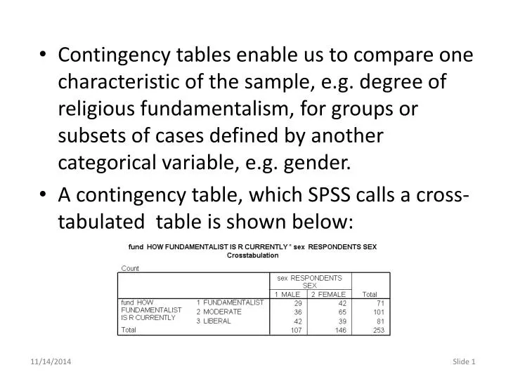
Contingency tables enable us to compare one characteristic of the sample, e.g. degree of religious fundamentalism, for groups or subsets of cases defined by another categorical variable, e.g. gender. • A contingency table, which SPSS calls a cross-tabulated table is shown below:
Each cell in the table represents a combination of the characteristics associated with the two variables: 29 males were also fundamentalists. 42 females were fundamentalists. While a larger number of females were fundamentalist, we cannot tell if females were more likely to be fundamentalist because the total number of females (146) was different from the total number of males (107). To answer the “more likely” question, we need to compare percentages.
There are three percentages that can be calculated for a contingency table: • percentage of the total number of cases • percentage of the total in each row • percentage of the total in each column • Each of the three percentages provide different information and answer a different question.
The percentage of the total number of cases is computed by dividing the number in each cell (e.g. 29, 42, etc.) by the total number of cases (253). 11.5% of the cases were both male and fundamentalist. 16.6% of the cases were both female and fundamentalist. We have two clues that the table contains total percentages. First, the rows that the percentages are on are labeled “% of Total.” Second, the 100% figure appears ONLY in the grand total cell beneath the table total of 253.
The percentage of the total for each row is computed by dividing the number in each cell (e.g. 29, 42) by the total for the row (71). 40.8% of the fundamentalists were male. 59.2% of the fundamentalists were female. The label for the percentage tells us that it is computed within the category for fundamentalist. The percentages in each row sums to 100% in the total column for rows (the row margin).
The percentage of the total for each column is computed by dividing the number in each cell (e.g. 29, 36, and 42) by the total for the column (107). 27.1% of the males were fundamentalists. 33.6% of the males were moderates. The label for the percentage tells us that it is computed within the category for sex. The percentage in each column sums to 100% in the total row for columns (the column margin).
The three percentages tell us: • the percent that is in both categories (total percentage) • the percent of each row that is found in each of the column categories (row percentages) • the percent of each column that is found in each of the row categories (column percentages) • The row and column percentages are referred to as conditional or contingent percentages.
The three percentages tell us: • the percent that is in both categories (total percentage) • the percent of each row that is found in each of the column categories (row percentages) • the percent of each column that is found in each of the row categories (column percentages) • The row and column percentages are referred to as conditional or contingent percentages.
Our real interest is in conditional or contingent percentages because these tell us about the relationship between the variables. • The relationship between variables is defined by a distinct role for each: • the variable which affected or impacted by the other is the dependent variable • the variable which affects or impacts the other is the independent variable • We assign the role to the variable. An independent variable in one analysis may be a dependent variable in another analysis.
A categorical variable has a relationship to another categorical variable if the probability of being in one category of the dependent variable differs depending on the category of the independent variable. • For example, if there is a relationship between social class and college attendance, the percentage of upper class persons who attend college will be different from the percentage of middle class persons who attend college. Attending college is the dependent variable and social class is the independent variable.
Given that we can represent this statistically with either the row or column percentages in a contingency table, my practice is to always put the independent variable in the columns and the dependent variable in the rows, and compute column percentages. • This order matches the order for many graphics where the dependent variable is on the vertical axis and the independent variable is on the horizontal axis.
Based on the column percentages, we can make statements like the following: Males were most likely to be liberal (39.3%), while females were most likely to be moderate (45.5%).
Based on the column percentages, we can make statements like the following: Males were more likely to be liberal (39.3%) compared to females (26.7%). This is not equivalent to the statement that liberals are more likely to be male or female.
We can also describe a relationship based on a comparison of odds. First, we compute the odds separately for each category of the independent variable: The odds that a female would be liberal rather than fundamentalist are 39 ÷ 42 = .93. The odds that a male would be a liberal rather than a fundamentalist are 42 ÷29 = 1.45.
We compare the odds by computing the ratio between the two: 1.45 for males ÷.93 for females = an odds ratio of 1.56. • We can now state the relationship between the two variables as: males are 1.56 times more likely to be liberal rather than fundamentalist, than are females. • This could also be stated as: being male increases the odds of being liberal rather than fundamentalist by a factor of 1.56 or 56%. (1.56 – 1.0 = .56) and multiplying .56 by 100 to convert it to a percent.
If the odds ratio were 1.0, then both groups would be equally likely to be liberals rather than fundamentalists. • We could have divided the odds for females by the odds for males (.93 ÷1.45 = .64) and stated that being female decreased the odds of being liberal versus fundamentalist by a factor of .64, or 36%. (.64 – 1.00 = .36) and multiplying .36 by 100 to convert it to a percent. Explaining decreases in odds is more awkward and less intuitive.
The introductory statement in the question indicates: • The data set to use (GSS200R) • The statistic to use (contingency table) • The variable to use in the rows of the table (attitude toward life ) • The variable to use in the columns of the table (sex)
The first statement for us to evaluate concerns the number of valid and missing cases. To answer this question, we produce the contingency table in SPSS.
To compute a contingency table in SPSS, select the Descriptive Statistics > Crosstabs command from the Analyze menu.
First, move the row variable life to the Row(s) list box. Second, move the column variable sex to the Column(s) list box. Third, click on Cells button to specify what should be printed in each cell of the table.
Second, click on the Continue button to close the dialog box. First, mark the check boxes for Column and Total percentages.
After returning to the Crosstabs dialog box, click on the OK button to produce the output.
The SPSS output provides us with the answer to the question on sample size. The 'Case Processing Summary' in the SPSS output showed the total number of valid cases to be 186 and the number of missing cases to be 84.
The 'Case Processing Summary' in the SPSS output showed the total number of valid cases to be 186 and the number of missing cases to be 84. Click on the check box to mark the statement as correct.
The next statement asks which combination of characteristics was most common. The key word and tell us that the problem is looking for total percentages, i.e. the percentage that has both characteristics.
The largest total percentage (30.1%) in the contingency table was in the cell for the column labeled FEMALE and the row labeled ROUTINE.
The statement that "more survey respondents were female and said that they generally find life pretty routine than any other combination of categories" is correct. The check box for the first statement is marked. Since this precludes the second statement from being marked, its checkbox is left unmarked.
The next pair of statements asks us to compare the groups, and identify which group was more likely (had a larger proportion) with the specified characteristic.
The column percent for survey respondents who were female was 54.4%, which was larger than the column percent of 44.6 for survey respondents who were male.
The statement that "compared to survey respondents who were male, those who were female were more likely to have said that they generally find life pretty routine" is correct. The check box for the first statement is marked. Since this precludes the second statement from being marked, its checkbox is left unmarked.
The next pair of questions gives two options for the most likely response for each group. The first option identifies alternatives for the most likely response. The second option states that both groups have the same most likely responses. The question of which response was most likely for each group requires that we identify the mode for each group.
The category EXCITING had the largest percentage of cases (49.4%), making it the modal category for survey respondents who were male.
The category ROUTINE had the largest percentage of cases (54.4%), making it the modal category for females.
The statement that "survey respondents who were male were most likely to have said that they generally find life exciting, while survey respondents who were female were most likely to have said that they generally find life pretty routine" is correct The check box for the first statement is marked. Since this precludes the second statement from being marked, its checkbox is left unmarked.
The final pair of questions requires us to compute the odds of describing life as routine rather than exciting for each group, and then compute the odds ratio to determine which group was more likely to have said life was routine rather than exciting.
The odds for survey respondents who were female was computed by dividing the ‘Count’ for ROUTINE by the ‘Count' for EXCITING (56÷44=1.27).
The odds for survey respondents who were male were computed by dividing the ‘Count' for ROUTINE by the ‘Count' for EXCITING (37÷41=0.90).
I use Excel to do the calculations that I cannot do easily in SPSS. First, I calculate the odds for each group (sex). Second, I calculate the odds ratio, once for the ratio of group 1 (females) to group 2 (males), and a second time for the ratio of group 2 (males) to group 1 (females). The odds ratio for females to males is 1.4, which corresponds to a greater likelihood for females.
The statement that "compared to survey respondents who were male, those who were female were about 1.4 times more likely to have said that they generally find life pretty routine" is correct. The odds for survey respondents who were female was computed by dividing the 'Count' for the ROUTINE row by the 'Count' for the EXCITING row in the FEMALE column (56÷44=1.27). The odds for survey respondents who were male was computed by dividing the 'Count' for the ROUTINE row by the 'Count' for the EXCITING row in the MALE column (37÷41=0.90). The odds ratio for survey respondents who were female to survey respondents who were male is 1.27 to 0.90, or 1.41 to 1. The second statement in the pair is marked.
The homework problems translate some of the decimal fractions for odds and odds ratios from numbers to text. The following table shows the translations used.
The homework problems translate some of the decimal fractions for odds and odds ratios from numbers to text. The following table shows the translations used.
After BlackBoard grades the assignment, it will give you an option to review the results. For this problem, we received the full 10 points because we marked all of the correct answers and did not mark any of the incorrect answers. Note: this version of BlackBoard does not give partial credit.
The feedback after the graded answer explains what the correct answer would have been.