But which line best describes our data?

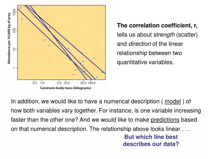
1. The correlation coefficient, r, tells us about strength (scatter) and direction of the linear relationship between two quantitative variables. In addition, we would like to have a numerical description ( model ) of how both variables vary together. For instance, is one variable increasing faster than the other one? And we would like to make predictions based on that numerical description. The relationship above looks linear . . . But which line best describes our data?

2. = - ˆ y 0 . 125 x 41 . 4 The regression line The least-squares regression line is the unique line such that the sum of the squares of the vertical distances of the data points to the line is the smallest possible.

3. And these equations are available in R through the function lm(y~x) ("lm" means "linear model"). Try lm on the manatee data… (manatee.csv)

4. = - ˆ y 0 . 125 x 41 . 4 The equation completely describes the regression line. To plot the regression line you only need to choose two x values, put them into the prediction equation, calculate y, and draw the line that goes through those two points... or let R do it for you with the abline function (abline(lm(y~x))) Hint: The regression line always passes through the mean of x and y. The points you use for drawing the regression line are computed from the equation. .125*450-41.4 = 14.85 .125*700-41.4= 46.1 So plot the points (450,14.85) & (700,46.1) X X

5. Hubble telescope data about galaxies moving away from earth: These two lines are the two regression lines calculated either correctly (x = distance, y = velocity, solid line) or incorrectly (x = velocity, y = distance, dotted line). The distinction between explanatory and response variables is crucial in regression. If you exchange y for x in calculating the regression line, you will get a different line. Regression examines the distance of all points from the linein the y direction only.

6. = - ˆ y 0 . 125 x 41 . 4 = - ˆ y 0 . 125 x 41 . 4 (in 1000’s) There is a positive linear relationship between the number of powerboats registered and the number of manatee deaths. The least squares regression line has the equation: Thus if we were to limit the number of powerboat registrations to 500,000, what could we expect for the number of manatee deaths? Roughly 21 manatees - do this with R using the predict function (see help(predict))

7. The least-squares regression line of y on x is the line that minimizes the sum of the squares of the vertical distances of the data points to the line. • The equation of the l-s line is usually represented as = b0 + b1 x where = the predicted value of y b0 = the intercept (predicted value of y when x=0) b1 = the slope of the prediction line • The correlation coefficient, r, is related to the l-s regression line as follows: the square of r (r2) is equal to the fraction of the variation in the values of the response variable y that is explained by the least squares regression of y on x. (See next slide)

8. Here are two plots of height (response) against age (explanatory) of some children. Notice how r2 relates to the variation in heights... r=0.994, r-square=0.988 r=0.921, r-square=0.848

9. Homework: • Read pages 8-10 in the Reading & Problems 2.1 on Linear Regression • note the R functions used here: model1=lm(y~x) plot(x,y) ; abline(model1) plot(model1) coef(model1) ; resid(model1) ; fitted(model1) plot(fitted(model1),resid(model1)) • Read at least one of the online sources for simple linear regression ( I like the second one…) http://www.stat.yale.edu/Courses/1997-98/101/linreg.htm http://www.statisticalpractice.com/ http://onlinestatbook.com/rvls/ http://www.sportsci.org/resource/stats/index.html

10. Homework(cont.) • FPG (mg/ml) - fasting plasma glucose (measured at home) HbA (% - measured in doctor's office). Can you predict FPG by HbA? Plot, compute the correlation coefficient, compute and plot the regression line and get a residual plot. Are there any unusual cases? Influential Points? Outliers?