Download

1 / 25
250 likes | 458 Views
Parameterizations of Resolved-Flow Driven Mixing and Planetary Boundary Layers. Simulated Kelvin-Helmholtz instability. 0.5. 0. Temperature (°C). z (m). -0.5. 0. -0.02. 0.02. u (m s -1 ). x. What is stratified shear mixing?.

E N D
Parameterizations of Resolved-Flow Driven Mixing and Planetary Boundary Layers
Simulated Kelvin-Helmholtz instability 0.5 0 Temperature (°C) z (m) -0.5 0 -0.02 0.02 u (m s-1) x What is stratified shear mixing? • When vertical shears of velocity are large enough, enough kinetic energy can be released by mixing to overcome the potential energy increase due to mixing against a density stratification, and mixing can spontaneously arise. • The necessary condition for instability is given by the shear Richardson number:
Where does stratified shear mixing matter in the ocean? • Dense overflows • Most interior ocean watermasses form through dense overflows. • Abyssal cataracts • Equatorial Undercurrent • The equatorial current and density structure are critical for ENSO. • Base of the surface mixed-layer • Property fluxes into the interior through non-deepening mixed layers may are important. • Wherever internal gravity waves steepen and break (maybe). • Critical slopes? • Parametric Subharmonic Instability (PSI)? All of these regions are important in the performance of large-scale ocean models, and need to be parameterized. The parameterization of resolved-flow driven mixing must be the same for all regions!
Shear-driven mixing of stratified turbulence Observed profiles from Red Sea plume from RedSOX (Peters and Johns, 2005) Actively mixing interfacial layer Shear param. appropriate here. Well-mixed bottom boundary layer (see Legg et al. 2006)
Abyssal Overflows – the Romanche Fracture Zone Potential Temperature along Romanche Fracture Zone Climatological Potential Temperature at 5000 m Depth Ferron et al., JPO 1998
Equatorial Undercurrent Shear Mixing Eastern Pacific Wind stress Western Pacific Westward Current in Surface Mixed Layer Eastward Equatorial Undercurrent Isotherms Side view along the equator
Impact of Shear-Mixing Parameterization on the EUC June Pacific EUC with Ricrit = 0.8 and Eo = 0.1 (Original values) Annual Mean Pacific EUC Ricrit = 0.2 and Eo = 0.005
Shear-mixing at the base of the mixed layer Wind Stress & TurbulentStress Density Velocity Sea surface Mechanical Stirring Shear mixing? Depth Stratified shear mixing at the base of the surface mixed layer figures prominently in such idealized mixed layer models as Pollard, Rhines & Thompson (1973) or Price, Weller & Pinkel (1986)
Shear-related mixing due to internal waves hitting a slope (Sonya Legg, Princeton U.)
Failure and Success of Existing Shear Mixing Parameterizations • A universal parameterization can have no dimensional “constants”. • KPP’s interior shear mixing (Large et al., 1994) and Pacanowski and Philander (1982) both use dimensional diffusivities. • The same parameterization should work for all significant shear-mixing. • In GFDL’s GOLD-based coupled model, Hallberg (2000) gives too much mixing in the Pacific Equatorial Undercurrent or too little in the plumes with the same settings. • To be affordable in climate models, must accommodate time steps of hours. • Longer than the evolution of turbulence. • Longer than the timescale for turbulence to alter its environment. • Existing 2-equation (e.g. Mellor-Yamada, k-, or k-w) closure models may be adequate. • The TKE equations are well-understood, but the second equation (length-scale, TKE dissipation, or TKE dissipation rate) tend to be ad-hoc (but fitted to observations) • Need to solve the vertical columns implicitly / iteratively in time for: • TKE • TKE dissipation / TKE dissipation rate / length-scale • Stratification (T & S) • (and 5.) Shear (u & v) • Simpler sets of equations may be preferable. • Many use boundary-layer length scales (e.g. Mellor-Yamada) and are not obviously appropriate for interior shear instability. • However, sensible results are often obtained by any scheme that mixes rapidly until the Richardson number exceeds some critical value. (e.g., Yu and Schopf, 1997)
Two-equation turbulence closures (At least) two equations for dimensional quantities are needed to describe turbulent mixing generically. One is the turbulent kinetic energy per unit mass (TKE) equation: With the usual Fickian (diffusive) closure it is And with small aspect ratio e≡ Dissipation of Q There are many options for the second equation, all very empirical: TKE-dissipation(k-e) TKE-dissipation rate(k-w) Mellor-Yamada 2.5
The second equation – e.g. TKE & dissipation (k-e) • TKE dissipation is (in)directly measurable. • None of the terms in a dissipation equation are measurable. • The functional form is chosen to mimic the TKE equation itself, with plenty of empirical constants added, mostly using boundary layer data. e≡ Dissipation of Q The n#m#, and d# are empirical constants. See Umlauf & Burchard (Cont. Shelf Res., 2005) for a review.
0.12 0.09 0.06 0.03 0 0 0.1 0.2 0.3 0.4 Entrainment-law Derived Parameterization for Shear-driven Mixing(L. Jackson, R. Hallberg, & S. Legg, JPO 2008) At boundaries: Diffusivity: k = 0 TKE/mass:Q = Q0 (≈ 0) F(Ri) Ri • Properties: • Simple enough to solve iteratively along with its impacts. • Complete enough to capture the essence of stratified shear instability. • Uses a length scale which is a combination of the width of the low Ri region (where F(Ri)>0), the buoyancy length scale LBuoy = Q1/2/N, and the distance from the boundary z-D. • Decays exponentially away from low Ri region. • Vertically uniform, unbounded limit: • Ellison and Turner limit (large Q): reduces to form similar to ET parameterization • Unstratified limit: similar to law-of-the-wall theories k [m2 s-1]Shear-driven diapycnal diffusivity / viscosity (Assumes Prandtl Number = 1) Q [m2 s-2] Turbulent kinetic energy per unit mass N2 = -g/r∂r/∂z [s-2]Buoyancy Frequency l, cN, cS [ ] Dimensionless (hopefully universal) constants
Simulated Shear-Driven Mixing Kelvin-Helmholtz instability 3D stratified turbulence z z x x
DNS data ET parameterisation JHL parameterisation RiCr = 0.25, cN = 0.30, cS = 0.11, = 0.85 RiCr = 0.30, cN = 0.25, cS = 0.11, = 0.79 RiCr = 0.35, cN = 0.24, cS = 0.12, = 0.80
DNS data ET parameterisation JHL parameterisation RiCr = 0.25, cN = 0.30, cS = 0.11, = 0.85 RiCr = 0.30, cN = 0.25, cS = 0.11, = 0.79 RiCr = 0.35, cN = 0.24, cS = 0.12, = 0.80
Comparison to other two-equation turbulence models Shear results JHL Jet results
Wind stirring-driven entrainment Conversion of resolved shears to small-scale turbulence (Richardson number criteria) Convective deepening Overshooting convective plumes Buoyancy-forced retreat to a Monin-Obuhkov depth Penetrating shortwave radiation Vertical decay of TKE Restratification due to ageostrophic shears in mixed layer (Ekman-driven, eddy-driven, and viscous stresses on thermal wind shears) Mostly at the base of the mixed layer and in the underlying transition layer. A “refined” bulk mixed layer, with vertical structure to the velocity in the mixed layer captures these processes (Hallberg, 2004) Important Processes for Determining Mixed Layer Depth
ASREX Mixed Layer Observations(Figures courtesy A. Gnanadesikan) • Is the bulk model’s fundamental assumption that the mixed layer is well mixed valid? • Mixed layers do tend to be well mixed in properties such as temperature. • Momentum is not well mixed, giving Ekman spirals with enough averaging. • The TKE budget formalism for a bulk mixed layer is probably not too bad.
A mixed layer TKE budget Bulk mixed layer entrainment is governed by a Turbulent Kinetic Energy balance: The mn are efficiencies and/or vertical decay of TKE. m2 is well known (1 or ~.2), while the others are not. • Many climate models use KPP, which effectively uses TKE balance considerations to determine the mixed layer depth and diffusivity profiles. Others use TKE budgets more directly. • Within the mixed layer, from law-of-the-wall and dimensional analysis, viscosity goes as
1-D Mixed Layer Simulations of SST at Bermuda 0.1 m Resolution KPP vs. 10 m Resolution KPP vs.GOLD with 63 layers High-frequency specified-flux forcing, including diurnal cycle, from BATS. Equivalent initial conditions. Sea Surface Temperature Mixing Layer Depth
Summary Surface Planetary Boundary Layer: Several approaches seem to work well enough • KPP • 2-Equation turbulence closures • Bulk mixed layers Resolved-shear mixing: • Many existing parameterizations in climate models are indefensible. • Better forms may exist, but the most important open questions arise from limited climate model resolutions.