Download
1 / 57
570 likes | 574 Views
Evolution of Life on Exoplanets and SETI (Evo-SETI). Claudio Maccone Director for Scientific Space Exploration, Int’l. Acad. Astronautics, Chair of the SETI Permanent Committee of the IAA, Associate, Istituto Nazionale di Astrofisica (INAF), Italy

E N D
Evolution of Lifeon Exoplanets and SETI(Evo-SETI) Claudio Maccone Director for Scientific Space Exploration, Int’l. Acad. Astronautics, Chair of the SETI Permanent Committee of the IAA, Associate, IstitutoNazionale di Astrofisica (INAF), Italy E-mail :clmaccon@libero.it Home Page : www.maccone.com Presentation at the «SETI Italia 2016» Conference IASF-INAF Milano, Italy, May 11, 2016.
ABSTRACT SETI and ASTROBIOLOGY have long been regarded as two separate research fields. The growing number of discovered exoplanets of various sizes and characteristics, however, forces us to envisage some sort of CLASSIFICATION of exoplanets based on the question: where does a newly-discovered exoplanet stand ON ITS WAY TO DEVELOP LIFE ?This author has tried to answer this question in a mathematical fashion by virtue of his "Evo-SETI" (standing for "Evolution and SETI") mathematical model. The results were two papers published in the International Journal of Astrobiology, the first of which turned out to be the second most-widely read paper in the International Journal of Astrobiology in the year 2013. In this seminar the Evo-SETI mathematical model is described in mathematical detail for the benefit of researchers.
TALK’s SCHEME Part 1: The STATISTICAL DRAKE EQUATIONPart 2: LIFEis a b-LOGNORMAL in timePart 3: Darwinian EXPONENTIAL GROWTH Part 4: Geometric Brownian Motion (GBM) Part 5: CLADISTICS: Species = b-LOGNORMALSPart 6: ENTROPY as EVOLUTION MEASUREPart 7: Mass Extinctions
The Classical Drake Equation /1 • In 1961 Frank Drake introduced his famous “Drake equation” described at the web site http://en.wikipedia.org/wiki/Drake_equation. It yields the number N of communicating civilizations in the Galaxy: • Frank Donald Drake (b. 1930)
The Classical Drake Equation /2 • The meaning of the seven factors in the Drake equation is well-known. • The middle factor fl is Darwinian Evolution. • In the classical Drake equation the seven factors are just POSITIVE NUMBERS. And the equation simply is the PRODUCT of these seven positive numbers. • It is claimed here that Drake’s approach is too “simple-minded”, since it does NOT yield the ERROR BAR associated to each factor!
The STATISTICAL Drake Equation /1 • If we want to associate an ERROR BAR to each factor of the Drake equation then… • … we must regard each factor in the Drake equation as a RANDOM VARIABLE. • Then the number N of communicating civilizations also becomes a random variable. • This we call the STATISTICAL DRAKE EQUATION and studied in our mentioned reference paper of 2010 (Acta Astronautica, Vol. 67 (2010), pages 1366-1383)
The STATISTICAL Drake Equation /2 • Denoting each random variable by capitals, the STATISTICAL DRAKE EQUATION reads • Where the D sub i (“D from Drake”) are the 7 random variables, and N is a random variable too (“to be determined”).
Generalizing the STATISTICAL Drake Equation to ANY NUMBER OF FACTORS /1 • Consider the statistical equation • This is the generalization of our Statistical Drake Equation to the product of ANY finite NUMBER of positive random variables. • Is it possible to determine the statistics of N ? • Rather surprisingly, the answer is “yes” !
Generalizing the STATISTICAL Drake Equation to ANY NUMBER OF FACTORS /2 • First, you obviously take the natural log of both sides to change the finite product into a finite sum • Second, to this finite sum one can apply the CENTRAL LIMIT THEOREM OF STATISTICS. It states that, in the limit for an infinite sum, the distribution of the left-hand-side is NORMAL. • This is true WHATEVER the distributions of the random variables in the sum MAY BE.
Generalizing the STATISTICAL Drake Equation to ANY NUMBER OF FACTORS /3 • So, the random variable on the left is NORMAL, i.e. • Thus, the random variable N under the log must be LOG-NORMAL and its distribution is determined! • One must, however, determine the mean value and variance of this log-normal distribution in terms of the mean values and variances of the factor random variables. This is DIFFICULT. But it can be done, for example, by a suitable numeric code that this author wrote in MathCad language.
ConclusionThe number of Signaling Civilizations is LOGNORMALLY distributed • Our Statistical Drake Equation, now Generalized to any number of factors, embodies as a special case the Statistical Drake Equation with just 7 factors. • The conclusion is that the random variable N (the number of communicating ET Civilizations in the Galaxy) is LOG-NORMALLY distributed. • The classical “old pure-number Drake value” of N is now replaced by the MEAN VALUE of such a log-normal distribution. • But we now also have an ERROR BAR around it !
REFERENCE PAPER : • The Statistical Drake Equation • Acta Astronautica, Vol. 67 (2010) p. 1366-1383.
Part 2:LIFE of a cell, of an animal, of a human, a civilization (f sub i) even ET (f sub L)is a b-LOGNORMALin time
LIFE is a FINITE b-LOGNORMAL • The lifetime of a cell, an animal, a human, a civilization may be modeled as a b-lognormal with tail REPLACED at senility by the descending TANGENT. The interception at time axis is DEATH=d.
LIFE is a FINITE b-LOGNORMAL • The equation of a INFINITE b-lognormal is : • The lifetime of a cell, an animal, a human, a civilization can be modeled as a FINITE b-lognormal: namely an infinite b-lognormal whose TAIL has been REPLACED at senility by the descending TANGENT STRAIGHT LINE. The interception of this straight line at time axis is DEATH=d.
Let a = increasing inflexion, s = decreasing inflexion. • Then any b-lognormal has birth time (b), adolescencetime (a), peak time (p) and senility time (s). • HISTORY FORMULAE : GIVEN (b, s, d) it is always possible to compute the corresponding b-lognormal by virtue of the HISTORY FORMULAE : LIFE as FINITE b-LOGNORMAL
Let a = increasing inflexion, s = decreasing inflexion. • Then any b-lognormal has birth time (b), adolescencetime (a), peak time (p) and senility time (s). • Rome’s civilization: b=-753, a=-146, p=59, s=235. LIFE as FINITE b-LOGNORMAL
Part 3:Darwinian EXPONENTIAL GROWTHas LOCUS of b-LOGNORMAL PEAKS
REFERENCE PAPER : • A Mathematical Model for Evolution and SETI • Origins of Life and Evolution of Biospheres (OLEB), Vol. 41 (2011), pages 609-619.
Darwinian EXPONENTIAL GROWTH • Life on Earth evolved since 3.5 billion years ago. • The number of Species GROWS EXPONENTIALLY: assume that today 50 million species live on Earth • Then:
Darwinian EXPONENTIAL GROWTH • Life on Earth evolved since 3.5 billion years ago. • The number of Species GROWS EXPONENTIALLY: assume that today 50 million species live on Earth • Then: • with:
Invoking b-LOGNORMALS i.e. LOGNORMALS starting at b =birth • b-lognormals are just lognormals starting at any finite positive instant b >0, that is supposed to be known. • b-lognormals are thus a family of probability density functions with three parameters: m, s, and b. • m and b are REAL variables, but s must be POSITIVE.
EXPONENTIAL as “ENVELOPE” of b-LOGNORMALS • Each b-lognormal has its peak on the exponential. • PRACTICALLY an “Envelope”.
b-LOGNORMAL PEAK /1 • QUESTION: Is it POSSIBLE to match the second equation (peak ordinate) with the EXPONENTIAL curve of the increasing number of Species ? • YES, by setting:
b-LOGNORMAL PEAK /2 • We noticed that it is POSSIBLE to MATCH these two equations EXACTLY just upon setting:
b-LOGNORMAL PEAK /3 • Moreover, the last two equations can be INVERTED, i.e. solved for m and s EXACTLY, thus yielding: • These two equations prove that, knowing the exponential (i.e. A and B) and peak time p, the b-lognormal HAVING ITS PEAK EXACTLY ON THE EXPONENTIALis perfectly determined (i.e. its m and s are perfectly determined given A, B and p. This is the BASIC RESULT to make further progress.
GEOMETRIC BROWNIAN MOTION(GBM): exponential mean value : GEOMETRIC BROWNIAN MOTIONlognormal probability density :
WARNING !!!GEOMETRIC BROWNIAN MOTIONis a WRONG NAME : This process in NOT a Brownian Motion at all since its probability density function is a LOGNORMAL, and NOT A GAUSSIAN !!! So, the pdf ranges between ZERO and INFINITY, and NOT between minus infinity and infinity!!! GBMs are the «Black-Sholes» Models in FINANCE.
GEOMETRIC BROWNIAN MOTIONis the extension in time of theSTATISTICAL DRAKE EQUATION: The two lognormals (of movie & picture) then COINCIDE.
In other words still:1) The CLASSICAL DRAKE EQ.is STATIC, and is a SUBSET of theSTATISTICAL DRAKE EQUATION.2) But in turn, the STATISTICAL DRAKE EQUATION is the STATIC VERSION(i.e. the STILL PICTURE) of the GEOMETRIC BROWNIAN MOTION(the MOVIE).
DARWINIAN EVOLUTION is a GBMin the increasing number of Species
DARWINIAN EVOLUTION is a GBMin the increasing number of Species
Part 5:CLADISTICS : Every new Species is a new b-lognormal
CLADISTICS : every new Species is just a new b-LOGNORMAL • Each b-lognormal has its peak on the exponential. • PRACTICALLY an “Envelope”, though not so formally.
A REFERENCE PAPER • Evolution and History in a new “Mathematical SETI” model. • ACTA ASTRONAUTICA, Vol. 93 (2014), pages 317-344. Online August 13, 2013.
Shannon ENTROPY for a probability density (in bits) : • Shannon ENTROPY for b-lognormals (in bits) b-LOGNORMAL ENTROPY
But m ONLY is a function of the peak abscissa p : • Shannon ENTROPY for any b-lognormal in bits b-LOGNORMAL ENTROPY
The ENTROPY DIFFERENCE among any two Civilizations having their two peak abscissae at p sub 1 and p sub 2 is given by • ENTROPY IS THUS A MEASURE OF THE LEVEL OF PROGRESS REACHED BY EACH CIVILIZATION. • ENTROPY DIFFERENCE measures the DIFFERENCE in civilization level among any two Civilizations. • If it is known WHEN the two Civilizations reached their two peaks, the above formula yields their CIVILIZATION LEVEL DIFFERENCE. CIVILIZATION LEVEL DIFFERENCE
EXAMPLES :CIVILIZATION DIFFERENCE • The DIFFERENCE in Civilization Level between the Spaniards and Aztecs in 1519 was about 3.84 bits per individual. • The DIFFERENCE in Civilization Level between a Victorian Briton and a Pericles Greek was about 1.76 bits per individual. • The DIFFERENCE in Civilization Level between Humanity and the first Alien Civilization we will find in the Galaxy is UNKNOWN, of course, but… • … but now we have a Mathematical Theory to ESTIMATE IT on the basis of the messages we get.
EXAMPLEEVOLUTION DIFFERENCE • The DIFFERENCE in Darwinian Evolution between two species on Earth is given by the same equation • The result is that the DIFFERENCE IN EVOLUTION LEVEL between the first living being 3.5 billion years ago – RNA - and Humans is about 25.57 bits per individual. • As for the DIFFERENCE in Civilization Level, except we must now use the different numerical value of Bthe enveloping Darwinian exponential, found earlier.
Evo-ENTROPYas INCREASING ORGANIZATION • We had to introduce Evo-ENTROPY as a measure of the ORGANIZATIONAL LEVEL of different SPECIES : • 1) We have dropped the MINUS SIGN in front of the Shannon Entropy in order to pass from a measure of disorganization (good for gases) to a measure of organization of the living SPECIES. • 2) We also wanted a straight line starting at zero at the time of the ORIGIN OF LIFE = -3.5 billion years.