Download
1 / 44
610 likes | 2k Views
Lecture 34: The Inverted Pendulum. This is just an upside down overhead crane. But first I’d like to review what we’ve been doing because I’m not sure we’re all getting it. Plus it will give us a nice point of reference before we go on. We’re looking at problems that can be reduced to

E N D
Lecture 34: The Inverted Pendulum This is just an upside down overhead crane But first I’d like to review what we’ve been doing because I’m not sure we’re all getting it Plus it will give us a nice point of reference before we go on We’re looking at problems that can be reduced to finding u such that some x goes to zero
picture/prose/?? differential equations in state space simulation linear equations QUESTIONS?! control algorithm verification
differential equations in state space Euler-Lagrange equations (second order) Convert to state space (first order) Add other equations as necessary (as in magnetic suspension)
Make the state equations formally a function of time simulation explicit time dependence is rare we won’t see it F is is a nonlinear vector Use some software (Mathematica, MatLab, . . .) to integrate the system Design whatever you like for output pictures
Find the equilibrium, a state such that F(xeq) = 0 Linearize the nonlinear equations in state space (around the equilibrium state) linear equations Find the A matrix and the B vector I generally drop the prime at this point so I don’t have to carry it around
Check for controllability: find S If controllable control algorithm
negative feedback Find gains in z space Characteristic polynomial control algorithm Desired characteristic polynomial Equate coefficients to determine the gains
control algorithm Does this work? We know the linear one will work We need to verify if the nonlinear one works
Why do we go to the bother of putting the system in companion form? Couldn’t we find gains directly in x space without all this extra work?
Yes, we could, but it’s not a great idea because We need to find S to figure out if the system is controllable No point is wasting time trying to find a control if it’s impossible The gain equations in z space separate: each equation has only one gain in it They do not separate if you try to solve directly in x space The bigger the system, the more valuable this help is Let me jump the gun and show you a slide I will show again later
The equations I need to solve are Each equation contains only one gain, making them trivial to solve
Now let’s look at the inverted pendulum which is just the overhead crane upside down
The overhead crane y M Turn this upside down to get the inverted pendulum Wheels roll without slipping Torque is applied to the rear wheel Neglect the inertia of the wheels Denote wheel radius by r q m (y1, z1)
(y1, z1) m q We can copy the development from the overhead crane M y
Energies Constraints The only difference is in the sign in thez constraint Lagrangian Generalized forces
Write the torque as that from a DC motor but we include the effects of induction on the current torque rotation rate current We will use, K1 = K = K2 back emf voltage = input voltage - back emf
Mechanical equations including the current Solve for the second derivatives And add the evolution equation for the current
Define a state vector The first two and last equations in the state are simple The other two use the separated second derivatives
All the derivatives of the state vector The forcing has moved to the new equation
I’m looking at the homogeneous case which I expect to be unstable
And it is unstable in a linear sense But the motor resistance eats up energy and the final state has no motion and the pendulum hanging down in its stable position and the cart in its initial position
Final state for the unforced inverted pendulum M y (y1, z1) m
So at this point we have found the equations of motion converted them to state space form and built and tested a simulation The next thing we need to do is linearize the system so that we can start down the road to control a nonlinear term, hence negligible standard trig reductions
1 0 Apply the linearization q 1 Linearized differential equations Solve for the second derivatives
We still need a fifth differential equation for the current it’s already linear so we can use the one we already have
Let’s look at the alternate linearization mechanism The Mathematica code Find the A matrix and the B vector
The results We see that the system is unstable in the linear sense
Now we want to determine controllability and, if it is controllable, find the gains required to control it controllable
We have the ritual we need to find T, A1 and B1 We’ll look at the details when we go through the Mathematica notebook
We have T where Li takes the place of the variable “inductance”
The upper part of A1 always looks like this If yours doesn’t, you’ve made a mistake somewhere We get: If you want another check on your work, find the eigenvalues of this matrix They should be the same as those of A
We want to find gains in z space that give us stable poles We want the eigenvalues of A1 – B1Gz to be the desired poles We compare the ideal characteristic polynomial to the characteristic polynomial of A1 – B1Gz The former is We can find the latter either by brute force and awkwardness or by taking advantage of the form of A1
brute force and awkwardness using the coefficients of A1
The equations I need to solve are Each equation contains only one gain, making them trivial to solve
This is about as far as it makes sense to go without putting in the numbers We have one sanity check available: if we put in the original eigenvalues do we get zero gain?
So now we have the question of where to put the poles: Should we just move the zero and unstable poles or should we go to a Butterworth configuration? We can try all of these in the notebook, but I’ll just look at the Butterworth result here We have five variables, so we need five poles, and the Butterworth five can be found from
We map poles into complex space to give us the gains We need to remember to map the gains into x space before simulation
And here is a result Cart originally 5 m to left of its desired location with the pendulum erect
Now let’s look at the whole thing in Mathematica but first QUESTIONS?!