Download
1 / 51
510 likes | 688 Views
Functional Mapping A statistical model for mapping dynamic genes. Recall: Interval mapping for a univariate trait. Simple regression model for univariate trait. Phenotype = Genotype + Error y i = x i j + e i. x i is the indicator for QTL genotype

E N D
Functional MappingA statistical model for mapping dynamic genes
Recall: Interval mapping for a univariate trait Simple regression model for univariate trait Phenotype = Genotype + Error yi = xij + ei xiis the indicator for QTL genotype jis the mean for genotype j ei ~ N(0, 2) ! QTL genotype is unobservable (missing data)
Overall trait distribution Qq QQ qq A simulation example (F2) The overall trait distribution is composed of three distributions, each one coming from one of the three QTL genotypes, QQ, Qq, and qq.
Solution: consider a finite mixture model With QQ=m+a, Qq=m+d, qq=m-a
We use finite mixture model for estimating genotypic effects (F2) yi ~ p(yi|,) = 2|if2(yi) + 1|if1(yi) + 0|if0(yi) QTL genotype (j) QQQqqq Code 210 where • fj(yi) is a normal distribution density • with mean jand variance 2 • = (2, 1, 0) = QTL conditional probability given on flanking markers
Human Development Robbins 1928, Human Genetics, Yale University Press
Tree growth Looks mess, but there are simple rules underlying the complexity.
The dynamics of gene expression • Gene expression displays in a dynamic fashion throughout lifetime. • There exist genetic factors that govern the development of an organism involving: • Those constantly expressed throughout the lifetime (called deterministic genes) • Those periodically expressed (e.g., regulation genes) • Also environment factors such as nutrition, light and temperature. • We are interested in identifying which gene(s) govern(s) the dynamics of a developmental trait using a procedure called Functional Mapping.
Stem diameter growth in poplar trees Ma et al. (2002) Genetics
Mouse growth A: male; B: female
QQ QQ Qq Qq QQ QQ Qq Qq Developmental Pattern of Genetic Effects Wu and Lin (2006) Nat. Rev. Genet.
Data Structure Parents AA aa F1Aa Aa F2AAAa aa ¼ ½ ¼
Mapping methods for dynamic traits • Traditional approach: treat traits measured at each time point as a univariate trait and do mapping with traditional QTL mapping approaches such as interval or composite interval mapping. • Limitations: • Single trait model ignores the dynamics of the gene expression change over time, and is too simple without considering the underlying biological developmental principle. • A better approach:Incorporate the biological principle into a mapping procedure to understand the dynamics of gene expression using a procedure calledFunctional Mapping(pioneeredby Wu and group).
A general framework pioneered by Dr. Wu and his colleagues, to map QTLs that affect the pattern and form of development in time course - Ma et al., Genetics 2002 - Wu et al., Genetics 2004 (highlighted in Nature Reviews Genetics) - Wu and Lin, Nature Reviews Genetics 2006 While traditional genetic mapping is a combination between classic genetics and statistics, functional mapping combines genetics, statistics and biological principles. Functional Mapping (FunMap)
Data structure for an F2 population Phenotype Marker _______________________________ ________________________________________ Sample y(1) y(2) … y(T) 1 2 … m _____________________________________________________________________________________ 1 y11 y21 … yT1 1 1 … 0 2 y12 y22 … yT2 -1 1 … 1 3 y13 y23 … yT3 -1 0 … 1 4 y14 y24 … yT4 1 -1 … 0 5 y15 y25 … yT5 1 1 … -1 6 y16 y26 … yT6 1 0 … -1 7 y17 y27 … yT7 0 -1 … 0 8 y18 y28 … yT8 0 1 … 1 n y1n y2n … yTn 1 0 … -1 ·There are nine groups of two-marker genotypes, 22, 21, 20, 12, 11, 10, 02, 01 and 00, with sample sizes n22, n21, …, n00; ·The conditional probabilities of QTL genotypes, QQ (2), Qq (1) and qq (0) given these marker genotypes 2i, 1i, 0i.
Univariate interval mapping L(y) = fj(yi) = j=2,1,0 for QQ, Qq, qq The Lander-Botstein model estimates (2, 1, 0, 2, QTL position) Multivariate interval mapping L(y) = Vector y = (y1, y2, …, yT) fj(yi) = Vectors uj = (j1, j2, …, jT) Residual variance-covariance matrix = The unknown parameters: (u2, u1, u0, , QTL position) [3T + T(T-1)/2 +T parameters]
Functional mapping: the framework Observed phenotype:yi = [yi(1), …, yi(T)] ~ MVN(uj, ) Mean vector: uj = [μj(1), μj(2), …, μj(T)], j=2,1,0 (Co)variance matrix:
Functional Mapping Functional mapping does not estimate (u2, u1, u0, ) directly, instead of the biologically meaningful parameters. An innovative model for genetic dissection of complex traits by incorporating mathematical aspects of biological principles into a mapping framework Provides a tool for cutting-edge research at the interplay between gene action and development
The Finite Mixture Model Three statistical issues: Modeling mixture proportions, i.e., genotype frequencies at a putative QTL Modeling the mean vector Modeling the (co)variance matrix
Modeling the developmental Mean Vector • Parametric approach Growth trajectories – Logistic curve HIV dynamics – Bi-exponential function Biological clock – Van Der Pol equation Drug response – Emax model • Nonparametric approach Lengedre function (orthogonal polynomial) Spline techniques
Example: Stem diameter growth in poplar trees Ma, et al. Genetics 2002
Logistic Curve of Growth – A Universal Biological Law (West et al.: Nature 2001) Instead of estimating mj, we estimate curve parameters p= (aj, bj, rj) Modeling the genotype- dependent mean vector, uj = [uj(1), uj(2),…, uj(T)] = [ , , …, ] Number of parameters to be estimated in the mean vector Time points Traditional approach Our approach 5 3 5 = 15 3 3 = 9 10 3 10 = 30 3 3 = 9 50 3 50 = 150 3 3 = 9
= Modeling the Covariance Matrix • Stationary parametric approach • Autoregressive (AR) model with log transformation • Nonstationary parameteric approach • Structured antedependence (SAD) model • Ornstein-Uhlenbeck (OU) process
Functional interval mappingL(y) = Vector y = (y1, y2, …, yk)f2(yi) = f1(yi) = f0(yi) = u2 = ( , ,…, )u1 = ( , , …, )u0 = ( , , …, )
The EM algorithm E step Calculate the posterior probability of QTL genotype j for individual i that carries a known marker genotype M step Solve the log-likelihood equations Iterations are made between the E and M steps until convergence
EM continued The likelihood function:
Statistical Derivations M-step: update the parameters (see Ma et al. 2002, Genetics for details)
Testing QTL effect: Global test • Instead of testing the mean difference at every time points for different genotypes, we test the difference of the curve parameters. • The existence of QTL is tested by • H0 means the three mean curves overlap and there is no QTL effect. • Likelihood ratio test with permutation to assess significance. where the notation “~” and “^” indicate parameters estimated under the null and the alternative hypothesis, respectively.
Testing QTL effect: Regional test • Regional test: to test at which time period [t1,t2] the detect QTL triggers an effect, we can test the difference of the area under the curve (AUC) for different QTL genotype, i.e., where • Permutation tests can be applied to assess statistical significance.
Applications • Several real examples are used to show the utility of the functional mapping approach. • Application I is about a poplar growth data set. • Application II is about a mouse growth data set. • Application III is about a rice tiller number growth data set.
Application I: A Genetic Studyin Poplars Parents AA aa F1Aa AA BC AAAa ½½ Genetic design
Stem diameter growth in poplar trees a: Asymptotic growth b: Initial growth r: Relative growth rate Ma, Casella & Wu, Genetics 2002
Differences in growth across ages Untransformed Log-transformed Poplar data
Modeling the covariance structure Stationary parametric approach First-order autoregressive model (AR(1)) Multivariate Box-Cox transformation to stabilize variance (Box and Cox, 1964 Transform-both-side (TBS) technique to reserve the interpretability of growth parameters (Carrol and Ruppert, 1984; Wu et al., 2004). For a log transformation (i.e., =0), q= (,2)
Results by FunMap Results by Interval mapping QTL Functional mapping incorporated by logistic curves and AR(1) model FunMap has higher power to detect the QTL than the traditional interval mapping method does. Ma, Casella & Wu, Genetics 2002
Application II: Mouse Genetic Study Detecting Growth Genes Data supplied by Dr. Cheverud at Washington University
Parents AA aa F1Aa Aa F2AAAa aa ¼ ½ ¼ Body Mass Growth for Mouse 510 individuals measured Over 10 weeks
Functional mappingGenetic control of body mass growth in mice Zhao, Ma, Cheverud & Wu, Physiological Genomics 2004
Application III: functional mapping of PCD QTL • Rice tiller development is thought to be controlled by genetic factors as well as environments. • The development of tiller number growth undergoes a process called programmed cell death (PCD).
Parents AA aa F1Aa DH AAaa ½½ Genetic design
Joint model for the mean vector • We developed a joint modeling approach with growth and death phases are modeled by different functions. • The growth phase is modeled by logistic growth curve to fit the universal growth law . • The dead phase is modeled by orthogonal Legendre function to increase the fitting flexibility.
Advantages of Functional Mapping Incorporate biological principles of growth and development into genetic mapping, thus, increasing biological relevance of QTL detection Provide a quantitative framework for hypothesis tests at the interplay between gene action and developmental pattern - When does a QTL turn on? - When does a QTL turn off? - What is the duration of genetic expression of a QTL? - How does a growth QTL pleiotropically affect developmental events? The mean-covariance structures are modeled by parsimonious parameters, increasing the precision, robustness and stability of parameter estimation
Functional Mapping:toward high-dimensional biology A new conceptual model for genetic mapping of complex traits A systems approach for studying sophisticated biological problems A framework for testing biological hypotheses at the interplay among genetics, development, physiology and biomedicine