Download
1 / 29
310 likes | 499 Views
Reduction of Temporal Discretization Error in an Atmospheric General Circulation Model (AGCM). Author: Daisuke Hotta hotta@umd.edu Advisor: Prof. Eugenia Kalnay Dept. of Atmospheric and Oceanic Science, University of Maryland, College Park ekalnay@atmos.umd.edu.

E N D
Reduction of Temporal Discretization Error in an Atmospheric General Circulation Model (AGCM) Author: Daisuke Hotta hotta@umd.edu Advisor: Prof. Eugenia Kalnay Dept. of Atmospheric and Oceanic Science, University of Maryland, College Park ekalnay@atmos.umd.edu
Numerical Weather Prediction (NWP):= Initial Value Problem of PDE Atmospheric Phenomena Governing Equations Numerical Discretization Solve ! (Simulate) from http://www.jma.go.jp/jma/jma-eng/jma-center/nwp/nwp-top.htm (Real Atmosphere) (from JMA website) Simulated Atmosphere from http://iprc.soest.hawaii.edu/news/news_2009.php O(109)-dimensional ODE Hydrodynamic PDE AGCM: Atmospheric General Circulation Model = a computer program which simulates the flow of global atmosphere by numerically integrating the governing fluid dynamical PDEs
Introduction: Motivation Due to computational restrictions … • most AGCMs adopt low-order time-integration schemes, such as • Leap-frog with Robert-Asselin filter (1st order) • Explicit Backward Euler (aka. Matsuno; 1storder) • Often, Δt is taken as the largest value for which computational instability is suppressed, • under the premise that temporal discretization errors are negligible compared to those associated with spatial discretization or Physical Parameterizations.
Introduction: Motivation However … • Spatial resolutions become finer and finer as the supercomputers become faster. • Is the premise justifiable ? • If not, how can we alleviate such errors ? Remedies (Approaches) : • Use a more accurate scheme with the same computational cost • Identify and parameterize the error, and reduce it using data assimilation
Approach 1 : A Better integration scheme (Lorenz N-cycle) Lorenz (1971) proposed an incredibly smart time-integration scheme which: • requires only 1 function evaluation per step • but yet (every N steps) it is of - (up to) 4th-order accuracy (for nonlinear systems) - arbitrary order of accuracy (for linear systems) However, this scheme seems to have remained forgotten. No applications have been made to AGCMs. Apply Lorenz N-cycle to an AGCM (Phase 1)
Approach 2: Estimation and Reduction of Model Errors Danforth et al. (2007) • Training: • Compute bias of the model error • Construct covariance matrix of the model state and the model error • Extract dominant modes using Singular Value Decomposition (SVD) • Model Error Reduction: • Estimate the model errors using bias statistics (state-independent) and regression in the space spanned by Singular Vectors (SVs) (state-dependent) • Reduce the error by subtracting the estimated error each time step during the integration Try this technique with an AGCM (Phase 2 & 3)
Phase 1: Approach • Implement Lorenz N-cycle to an existing AGCM • Implement 4th order Runge-Kutta as well as a reference • Compare the accuracy and efficiency of the newly introduced schemes with the original scheme
Phase 1: Algorithms ODE to be solved: (existing) Leap-frog with Robert-Asselin Filter Lorenz N-cycle 4th order Runge-Kutta Memory consumption: 2 x dim{model state} Memory consumption: 2 x dim{model state} Memory consumption: 5 x dim{model state} F-evaluation: 1per time step F-evaluation: 1per time step F-evaluation: 4 per time step accuracy: (N <= 4) O((NΔt)N)(every N steps) O(NΔt )(in between) accuracy: O(Δt4) accuracy: O(Δt )
AGCM: SPEEDY model • A fast AGCM with simplified physical parameterizations • Developed in Italy by Drs. F. Molteni and F. Kucharski • Horizontal Discretization: Spectral Representation with Spherical Harmonics truncated at total wavenumber 30 (T30) • Vertical Discretization: 8-layers Finite Difference on σ-coordinate • Temporal Discretization: Leap-Frog scheme with Robert-Asselin Filter (1st order Forward Euler for the physical parameterizations)
The equations solved:the “primitive” equation system (PDEs) on a spherical geometry + parametrized processes Sub-grid Parametrizations Dynamical Core …..
Spatial discretization:Spectral representation w.r.t. Spherical Harmonics • Spherical geometry: straightforwardly treated by spectral representation : • By the use of spherical harmonics expansion, differentiation becomes algebraic operation to the coefficients • e.g. Laplacian images taken from http://en.wikipedia.org/Spherical_harmonics
AGCM: SPEEDY model • Model Output • = (simulated) Global Weather or Climate Simulated Winter Precipitation (rain fall) Observed Winter Precipitation (rain fall) Images cited from http://users.ictp.it/~kucharsk/speedy8_clim_v41.html
AGCM: SPEEDY model • Language: Fortran77 • Platform: Any machine which supports Fortan77 compiler (a Linux server will be used in this study) • Code statistics: ~10,000 lines, 73 files • # predicted variables: ~ O(105) Implementation to be made: • Add new subroutines for N-cycle schemes and 4thorder Runge-Kutta scheme (for validation) • Add an Option to Switch-off Physical Parameterizations • Add an Option to run with flat orography
Phase 1: Issues to be avoided • Complications due to Physical Parameterizations: • Physical parameterizations include discontinuous processes (such as “if”-branches). • Avoid complications by switching-off parameterizations in the validations
Phase 1: Validation and Testing • Compare the new code with the original code • Switch-off parametrizations, remove orography (mountains), and perform Jablonowski-Williamson dynamical core tests (Jablonowski 2006): • Steady-state test case: start from steady-state initial condition, and see if the model can maintain that state. • Baroclinic wave test case: run the model from a specified initial condition. Analytical solution does not exist, but a reference solution (with uncertainty range) is available.
Phase 1: Database • Reference Solutions for the Jablonowski-Williamson Baroclinic wave test case • available from the University of Michigan website • http://esse.engin.umich.edu/groups/admg/ASP_Colloquium.php • http://www-personal.umich.edu/~cjablono/dycore_test_suite.html • Generated from 4 high-resolution models (approx. 50km mesh) • Uncertainty estimate evaluated as the difference among those high-resolution models is also available.
Phase 1: Validation (detail) • Run the models, with the originalscheme (Leap-Frog) and the new schemes (Runge-Kutta 4th and Lorenz N-cycle), from the specified initial condition. • Compute RMS difference of the surface pressure with respect to the reference solution. • If the new schemes are no further to the reference solution than to the original scheme, we can conclude that the implementation is successful.
Plot the RMS difference ||ps– psREF|| If the plot looks like below: Success If the plot looks like below: Failure Original New New Original Uncertainty Estimate Uncertainty Estimate
Approach 2: Estimation and Reduction of Model Errors Danforth et al. (2007) • Training: • Compute bias of the model error • Construct covariance matrix of the model state and the model error • Extract dominant modes using Singular Value Decomposition (SVD) • Model Error Reduction: • Estimate the model errors using bias statistics (state-independent) and regression in the space spanned by Singular Vectors (SVs) (state-dependent) • Reduce the error the model state through nudging each time step during the integration Try this technique with an AGCM (Phase 2 & 3)
Phase 2: Approach • Take the Truth from NCEP/NCAR reanalysis (Kalnay et al. 1996) NCEP=National Centers for Environmental Prediction NCAR=National Center for Atmospheric Research • Extract model errors by applying the method of Danforth et al. (2007) to the models with: • the original scheme (Leap-Frog; MLF) • Runge-Kutta 4thorder scheme (MRK4) • Lorenz N-cycle scheme (MNCYC) • (time permitting) Correct the model errors on-line during the course of model integration ( Phase 3&4)
Phase 2: Algorithm • Generate initial values from the Truth (NCEP/NCAR reanalysis) • Perform short-range forecasts using the 3 models (MLF, MRK4, MNCYC4) from the initial conditions • find the bias of the model errors for each model • Build the covariance matrix • Extract the dominant modes by conducting SVD
Phase 2: Implementation • Programs to be implemented: • computation of the bias and the covariance matrix • a program to perform SVD to the covariance • Platform: Linux server on AOSC dept.’s network • Language: Fortran90
Phase 2: Validation • For the SVD code: • Prepare a small-dimensional dummy data and run the program for this small data • Check if the result agrees with the result obtained by Matlab package. • For the entire implementation: Check if the the model errors obtained for MLF agrees with Danforth et al. (2007)
Phase 2: Testing (Verification) • Compare the amplitude of model errors (bias and covariance) for the new schemes (MRK4 and MNCYC) with those for the original scheme MLF • If the errors are smaller for the new schemes Successful • Otherwise Unsuccessful
Deliverables Phase 1: • Upgraded code for SPEEDY model - subroutines for Lorenz N-cycle and 4th order Runge-Kutta • Test-case results for the SPEEDY model (both for the original scheme and the new schemes) Phase 2: • Archive of the model errors • Pairs of Singular Vectors for the model state and the model error • Code for performing SVD
Schedule and Milestones Phase 1: Phase 2: • Implement RK4 and N-cycle, Nov. • Write the mid-year report, prepare the oral presentation, Dec. • Switch-off physical parameterizations, prepare flat topography, Jan. • perform the dynamical core tests. Feb. • Generate initial values from the NCEP/NCAR reanalysis, end of Feb. • build the bias and covariance matrix, Mar. • Code and test a program for SVD, Apr. • Compare the model errors for the new and the original shcmes, May. • Write the final report, May.
Phase 3(If time allows): Model Correction • During the integration of MLF, on each time step, • Correct the model bias within the model. • estimate the model error by regressing the model state onto the model error in the space spanned by the SVs. • Correct the 1-step forecast by subtracting the estimated error
Phase 4 (if time allows): Repeat Phase 2&3 with data assimilation • Generate nature-run by running MRK4 • Add random numbers to the nature-run to generate pseudo-observations • Perform data assimilation with SPEEDY-LETKF (Miyoshi 2005) • Compute the model error assuming the analysis is the truth, and repeat Phase 2 & 3
Bibliography Lorenz N-cycle • Lorenz, Edward N., 1971: An N-cycle time-differencing scheme for stepwise numerical integration. Mon. Wea. Rev., 99, 644–648. SPEEDY model • Molteni, Franco, 2003: Atmospheric simulations using a GCM with simplified physical parameterizations. I. Model climatology and variability in multi-decadal experiments. Clim. Dyn., 20, 175-191. • Kucharski F, Molteni F, and BraccoA, 2006: Decadal interactions between the western tropical Pacific and the North Atlantic Oscillation. Clim. Dyn., 26, 79-91 SPEEDY-LETKF • Miyoshi, T., 2005: Ensemble Kalman filter experiments with a primitive-equation global model. Ph.D. dissertation, University of Maryland, College Park, 197pp. Atmospheric GCM Dynamical Core test cases • Jablonowski, C. and D. L. Williamson 2006: A baroclinic instability test case for atmospheric model dynamical cores, Q. J. R. Metorol. Soc., 132, 2943-2975 NCEP/NCAR reanalysis • Kalnay, E., and Coauthors, 1996: The NCEP/NCAR 40-Year Reanalysis Project. Bull. Amer. Meteor. Soc., 77, 437–471. Model Error Correction • Danforth, Christopher M., Eugenia Kalnay, Takemasa Miyoshi, 2007: Estimating and Correcting Global Weather Model Error. Mon. Wea. Rev., 135, 281–299. • Danforth, Christopher M., Eugenia Kalnay, 2008: Using Singular Value Decomposition to Parameterize State-Dependent Model Errors. J. Atmos. Sci., 65, 1467–1478.